Solution manual microeconomics 7e by pindyck ch4
Bạn đang xem bản rút gọn của tài liệu. Xem và tải ngay bản đầy đủ của tài liệu tại đây (332.84 KB, 20 trang )
To download more slides, ebook, solutions and test bank, visit
Chapter 4: Individual and Market Demand
CHAPTER 4
INDIVIDUAL AND MARKET DEMAND
TEACHING NOTES
Chapter 4 builds on the consumer choice model presented in Chapter 3. Students find this
material very abstract and “unrealistic,” so it is important to convince them that there are good
reasons for studying how consumers make purchasing decisions in some detail. Most importantly, we
gain a deeper understanding of what lies behind demand curves and why, for example, demand curves
almost always slope downward. The utility maximizing model is also crucial in determining the supply
of labor in Chapter 14, general equilibrium in Chapter 16, and market failure in Chapter 18. So play
up these applications when selling students on the importance of the material in this chapter.
Section 4.1 focuses on graphically deriving individual demand and Engel curves by changing
price and income. Section 4.2 develops the income and substitution effects of a price change and
explains the (perhaps mythical) Giffen good case where the demand curve slopes upward. Section 4.3
shows how to derive the market demand curve from individuals’ demand curves. The remaining
sections cover consumer surplus, network externalities and empirical demand estimation
When discussing the derivation of demand, review how the budget line pivots around an
intercept as price changes and how optimal quantities change as the budget line pivots. Most of the
diagrams in the book analyze decreases in price, so you might want to go over an example in which
price increases. This will come in handy if you later go over the effects of a gasoline tax in Example
4.2. Once students understand the effect of price changes on consumer choice, they can grasp the
derivation of the price-consumption path and the individual demand curve. Remind students that the
price a consumer is willing to pay is a measure of the marginal benefit of consuming another unit. This
is important for understanding consumer surplus in Section 4.4
Income and substitution effects are difficult for most students, so spend some extra time going
over this material. Students frequently have trouble remembering which effect is which on the graph.
Emphasize that the substitution effect explains the change in quantity demanded caused by the
change in relative prices holding utility constant (a change in the slope of the budget line while staying
on the original indifference curve), while the income effect explains the change in quantity demanded
caused by a change in purchasing power (a shift of the budget line). Be sure to explain that the
substitution effect is always negative (i.e., relative price and quantity are negatively related). On the
other hand, the direction of the income effect depends on whether the product is a normal or inferior
good. It is a good idea to cover both a price increase and a price decrease.
If students are having trouble understanding the income effect, you might want to give a few
numerical examples of how purchasing power changes as the result of a price change. For example,
suppose a consumer typically buys a can of soda every day for $.75 per can. If the price increases to
$1.00, the consumer’s purchasing power drops by $.25, and she will have to spend less on other goods
and/or buy less soda. Over a month this amounts to a reduction in real income of roughly $.25 x 30 =
$7.50. You can show how the income effect can be large or small depending on how much the
consumer spends on the product and how much the price changes.
When covering the aggregation of individual demand curves in Section 4.3, stress that this is
equivalent to the horizontal summation of the individual demand curves because we want to add up
the quantities demanded by all consumers at each price. To obtain the market demand curve, you
must have demand written in the form Q = f(P) as opposed to the inverse demand P = f(Q). The
concept of a kink in the market demand curve is often new to students. Emphasize that this is because
not all consumers are in the market at all prices. With many consumers there can be many kinks.
With thousands of consumers, however, we hardly notice the individual kinks, so it is reasonable to
draw most market demand curves as smooth lines.
The concept of elasticity is reintroduced and further explored in Section 4.3. In particular, the
relationship between elasticity and revenue is explained.
49
Copyright © 2009 Pearson Education, Inc. Publishing as Prentice Hall.
To download more slides, ebook, solutions and test bank, visit
Chapter 4: Individual and Market Demand
Here is a way to help students remember this relationship. Think of price and revenue as being
connected by a link of some sort. If the link is elastic, price and revenue move in opposite directions
because the link between them stretches like a rubber band (for example, an increase in price leads to
a decrease in revenue), but if the link is inelastic, price and revenue must move in the same direction
because the link is rigid or inflexible.
Consumer surplus is introduced in Section 4.4. Emphasize that it measures the value a
consumer places on a good in excess of the price the consumer pays for the good. It is the difference
between what the consumer is willing to pay and what he or she actually has to pay for the good. We
usually measure consumer surplus using a market demand curve, in which case we are finding the
sum of all the individual consumer surpluses. Go over an example with a linear demand curve, and
remind students that the area of a triangle is (½)(base)(height). Example 4.5 is a nice application of
consumer surplus, but students have a hard time understanding the demand curve for reductions in
air pollution, so expect to spend some time if you cover this example. The related topic of producer
surplus is covered in Chapter 8, and both producer and consumer surplus are used extensively in
Chapter 9 and later chapters
Network externalities in Section 4.5 can be covered quickly, and they are pretty intuitive for
most students. Figures 4.16 and 4.17 are a bit complicated, but you do not have to cover them to get
the main points across. A nice example of a negative network externality that is covered only briefly in
the text is congestion. Road congestion is something most students can relate to, and you could
mention the comment about a popular NY City restaurant attributed to Yogi Berra that goes
something like, “It’s gotten so crowded, nobody goes there anymore.”
The first part of Section 4.6, “The Statistical Approach to Demand Estimation,” is fairly
straightforward, even if you have not covered the forecasting section of Chapter 2. It is important for
students to understand that demand curves really do exist and can be estimated. Many seem to think
demand curves are figments of economists’ imaginations and that we draw them more or less
randomly, so this part of the section is very useful. The second part, “The Form of the Demand
Relationship,” is more complicated and difficult for students who do not understand logarithms.
The Appendix is intended for students with a background in calculus. It goes through the
maximization of utility subject to a budget constraint using the Lagrange multiplier method. Demand
curves are derived and many of the conditions developed in Chapter 3 are shown mathematically.
There is a brief treatment of duality in consumer theory, and the mathematical form for the Slutsky
equation is discussed but not derived mathematically.
QUESTIONS FOR REVIEW
1. Explain the difference between each of the following terms:
a. a price consumption curve and a demand curve
The difference between a price consumption curve (PCC) and a demand curve is that
the PCC shows the quantities of two goods that a consumer will purchase as the price
of one of the goods changes, while a demand curve shows the quantity of one good
that a consumer will purchase as the price of that good changes. The graph of the
PCC plots the quantity of one good on the horizontal axis and the quantity of the
other good on the vertical axis. The demand curve plots the quantity of the good on
the horizontal axis and its price on the vertical axis.
b. an individual demand curve and a market demand curve
An individual demand curve plots the quantity demanded by one person at various
prices. A market demand curve is the horizontal sum of all the individual demand
curves for the product. It plots the total quantity demanded by all consumers at
various prices.
50
Copyright © 2009 Pearson Education, Inc. Publishing as Prentice Hall.
To download more slides, ebook, solutions and test bank, visit
Chapter 4: Individual and Market Demand
c. an Engel curve and a demand curve
An Engel curve shows the quantity of one good that will be purchased by a consumer
at different income levels. The quantity of the good is plotted on the horizontal axis
and the consumer’s income is on the vertical axis. A demand curve is like an Engel
curve except that it shows the quantity that will be purchased at different prices
instead of different income levels.
d. an income effect and a substitution effect
Both the substitution effect and income effect occur because of a change in the price
of a good. The substitution effect is the change in the quantity demanded of the good
due to the price change, holding the consumer’s utility constant. The income effect is
the change in the quantity demanded of the good due to the change in purchasing
power brought about by the change in the good’s price.
2. Suppose that an individual allocates his or her entire budget between two goods, food
and clothing. Can both goods be inferior? Explain.
No, the goods cannot both be inferior; at least one must be a normal good. Here’s why.
If an individual consumes only food and clothing, then any increase in income must be
spent on either food or clothing or both (recall, we assume there are no savings and
more of any good is preferred to less, even if the good is an inferior good). If food is an
inferior good, then, as income increases, consumption of food falls. With constant
prices, the extra income not spent on food must be spent on clothing. Therefore, as
income increases, more is spent on clothing, i.e. clothing is a normal good.
3. Explain whether the following statements are true or false.
a. The marginal rate of substitution diminishes as an individual moves
downward along the demand curve.
True. The consumer maximizes his utility by choosing the bundle on his budget line
where the price ratio is equal to the MRS. For goods 1 and 2, P1/P2 = MRS. As the
price of good 1 falls, the consumer moves downward along the demand curve for good
1, and the price ratio (P1/P2) becomes smaller. Therefore, MRS must also become
smaller, and thus MRS diminishes as an individual moves downward along the
demand curve.
b. The level of utility increases as an individual moves downward along the
demand curve.
True. As the price of a good falls, the budget line pivots outward, and the consumer
is able to move to a higher indifference curve.
c. Engel curves always slope upwards.
False. If the good is inferior, then as income increases, quantity demanded
decreases, and therefore the Engel curve slopes downwards.
4. Tickets to a rock concert sell for $10. But at that price, the demand is substantially
greater than the available number of tickets. Is the value or marginal benefit of an
additional ticket greater than, less than, or equal to $10? How might you determine that
value?
The diagram below shows this situation. At a price of $10, consumers want to purchase Q
tickets, but only Q* are available. Consumers would be willing to bid up the ticket price to
P*, where the quantity demanded equals the number of tickets available. Since utilitymaximizing consumers are willing to pay more than $10, the marginal increase in
satisfaction (i.e., the value or marginal benefit of an additional ticket) is greater than $10.
One way to determine the value of an additional ticket would be to auction it off.
51
Copyright © 2009 Pearson Education, Inc. Publishing as Prentice Hall.
To download more slides, ebook, solutions and test bank, visit
Chapter 4: Individual and Market Demand
Another possibility is to allow scalping. Since consumers are willing to pay an amount
equal to the marginal benefit they derive from purchasing an additional ticket, the scalper’s
price equals that value.
Price
Supply
P*
$10
Demand
Q*
Q
Tickets
5. Which of the following combinations of goods are complements and which are
substitutes? Can they be either in different circumstances? Discuss.
a. a mathematics class and an economics class
If the math class and the economics class do not conflict in scheduling, then the classes
could be either complements or substitutes. Math is important for understanding
economics, and economics can motivate mathematics, so the classes could be
complements. If the classes conflict or the student has room for only one in his
schedule, they are substitutes.
b. tennis balls and a tennis racket
Tennis balls and a tennis racket are both needed to play tennis, thus they are
complements.
c. steak and lobster
Foods can both complement and substitute for each other. Steak and lobster can be
substitutes, as when they are listed as separate items on a menu. However, they can
also function as complements because they are often served together.
d. a plane trip and a train trip to the same destination
Two modes of transportation between the same two points are substitutes for one
another.
e. bacon and eggs
Bacon and eggs are often eaten together and are complementary goods in that case.
However, in relation to something else, such as pancakes, bacon and eggs can function
as substitutes.
6. Suppose that a consumer spends a fixed amount of income per month on the following
pairs of goods:
a.
b.
c.
d.
tortilla chips and salsa
tortilla chips and potato chips
movie tickets and gourmet coffee
travel by bus and travel by subway
52
Copyright © 2009 Pearson Education, Inc. Publishing as Prentice Hall.
To download more slides, ebook, solutions and test bank, visit
Chapter 4: Individual and Market Demand
If the price of one of the goods increases, explain the effect on the quantity demanded of
each of the goods. In each pair, which are likely to be complements and which are likely
to be substitutes?
a. If the price of tortilla chips increases, the consumer will demand fewer tortilla
chips. Since tortilla chips and salsa are complements, the demand curve for salsa
will decrease (shift to the left), and the consumer will demand less salsa.
b. If the price of tortilla chips increases, the consumer will demand fewer tortilla
chips. Since tortilla chips and potato chips are substitutes, the demand for potato
chips will increase (the demand curve will shift to the right), and the consumer will
demand more potato chips.
c. The consumer will demand fewer movies after the price increase. You might think
the demands for movies and gourmet coffee would be independent of each other.
However, because the consumer spends a fixed amount on the two, the demand for
coffee will depend on whether the consumer spends more or less of her fixed budget
on movies after the price increase. If the consumer’s demand elasticity for movie
tickets is elastic, she will spend less on movies and, therefore, more of her fixed
income will be available to spend on coffee. In this case, her demand for coffee
increases, and she buys more gourmet coffee. The goods are substitutes in this
situation. If her demand for movies is inelastic, however, she will spend more on
movies after the price increase and, therefore, less on coffee. In this case, she will
buy less of both goods in response to the price increase for movies, so the goods are
complements. Finally, if her demand for movies is unit elastic, she will spend the
same amount on movies and therefore will not change her spending on coffee. In this
case, the goods are unrelated, and the demand curve for coffee is unchanged.
d. If the price of bus travel increases, the amount of bus travel demanded will fall,
and the demand for subway rides will rise, because travel by bus and subway are
substitutes. The demand curve for subway rides will shift to the right.
7. Which of the following events would cause a movement along the demand curve for
U.S. produced clothing, and which would cause a shift in the demand curve?
a. the removal of quotas on the importation of foreign clothes
The removal of quotas will allow U.S. consumers to buy more foreign clothing. Because
foreign produced goods are substitutes for domestically produced goods, the removal of
quotas will result in a decrease in demand (a shift to the left) for U.S. produced clothes.
There could be a smaller secondary effect also. When the quotas are removed, the total
supply of clothing will increase, causing clothing prices to fall. The drop in clothing
prices will lead consumers to buy more U.S. produced clothing, which is a movement
along the demand curve.
b. an increase in the income of U.S. citizens
When income rises, expenditures on normal goods such as clothing increase, causing
the demand curve to shift out to the right.
c. a cut in the industry’s costs of producing domestic clothes that is passed on to the
market in the form of lower prices
A cut in an industry’s costs will shift the supply curve out. The equilibrium price will
fall and quantity demanded will increase. This is a movement along the demand
curve.
53
Copyright © 2009 Pearson Education, Inc. Publishing as Prentice Hall.
To download more slides, ebook, solutions and test bank, visit
Chapter 4: Individual and Market Demand
8. For which of the following goods is a price increase likely to lead to a substantial
income (as well as substitution) effect?
a. salt
Small income effect, small substitution effect: The amount of income that is spent on
salt is very small, so the income effect is small. Because there are few substitutes for
salt, consumers will not readily substitute away from it, and the substitution effect is
therefore small.
b. housing
Large income effect, small substitution effect: The amount of income spent on housing is
relatively large for most consumers. If the price of housing rises, real income is
reduced substantially, leading to a large income effect. However, there are no really
close substitutes for housing, so the substitution effect is small.
c. theater tickets
Small income effect, large substitution effect: The amount of income spent on theater
tickets is relatively small, so the income effect is small. The substitution effect is large
because there are many good substitutes such as movies, TV shows, bowling, dancing
and other forms of entertainment.
d. food
Large income effect, virtually no substitution effect: As with housing, the amount of
income spent on food is relatively large for most consumers, so the income effect is
large. Although consumers can substitute out of particular foods, they cannot
substitute out of food in general, so the substitution effect is essentially zero.
9. Suppose that the average household in a state consumes 800 gallons of gasoline per
year. A 20-cent gasoline tax is introduced, coupled with a $160 annual tax rebate per
household. Will the household be better or worse off under the new program?
If the household does not change its consumption of gasoline, it will be unaffected by
the tax-rebate program, because the household pays ($0.20)(800) = $160 in taxes and
receives $160 as an annual tax rebate. The two effects cancel each other out.
However, the utility maximization model predicts that the household will not continue
to purchase 800 gallons of gasoline but rather will reduce its gasoline consumption
because of the substitution effect. As a Other Goods E
result, it will be better off after the tax
A
and rebate program. The diagram
shows this situation. The original
G
budget line is AD, and the household
maximizes its utility at point F where
OG
F
the budget line is tangent to
U2
indifference curve U1.
At F, the
U1
household consumes 800 gallons of
gasoline and OG of other goods. The
20-cent increase in price brought about
B 800
C
D
Gasoline
by the tax pivots the budget line to AB
(which is exaggerated to make the diagram clearer). Then the $160 rebate shifts the
budget line out in a parallel fashion to EC where the household is again able to
purchase its original bundle of goods containing 800 gallons of gasoline. However, the
new budget line intersects indifference curve U1 and is not tangent to it. Therefore,
point F cannot be the new utility maximizing bundle of goods. The new budget line is
tangent to a higher indifference curve U2 at point G. Point G is therefore the new
utility maximizing bundle, and the household consumes less gasoline (because G is to
the left of F) and is better off because it is on a higher indifference curve.
54
Copyright © 2009 Pearson Education, Inc. Publishing as Prentice Hall.
To download more slides, ebook, solutions and test bank, visit
Chapter 4: Individual and Market Demand
10. Which of the following three groups is likely to have the most, and which the least,
price-elastic demand for membership in the Association of Business Economists?
a. students
The major differences among the groups are the level of income and commitment to a
career in business economics. We know that demand will be more elastic (all else
equal) if a good’s consumption constitutes a large percentage of an individual’s income,
because the income effect will be large. Also demand is less elastic the more the good is
seen as a necessity. For students, membership in the Association is likely to represent
a larger percentage of income than for the other two groups, and students are less
likely to see membership as critical for their success. Thus, their demand will be the
most elastic.
b. junior executives
The level of income for junior executives will be larger than for students but smaller
than for senior executives. They will see membership as important but perhaps not as
important as for senior executives. Therefore, their demand will be less elastic than
students but more elastic than senior executives.
c.
senior executives
The high earnings among senior executives and the high importance they place on
membership will result in the least elastic demand for membership.
11. Explain which of the following items in each pair is more price elastic.
a. The demand for a specific brand of toothpaste and the demand for toothpaste in
general
The demand for a specific brand is more elastic because the consumer can easily
switch to another brand if the price goes up.
b. The demand for gasoline in the short run and the demand for gasoline in the long
run
Demand in the long run is more elastic since consumers have more time to adjust to
a change in price. For example, consumers can buy more fuel efficient vehicles, move
closer to work or school, organize car pools, etc.
12. Explain the difference between a positive and a negative network externality and
give an example of each.
A positive network externality exists if one individual’s demand increases in response
to the purchase of the good by other consumers. Fads are an example of a positive
network externality. For example, each individual’s demand for baggy pants
increases as more other individuals begin to wear baggy pants. This is also called a
bandwagon effect. Another example of a positive network externality occurs with
communications equipment such as telephones. A telephone is more desirable when
there are a large number of other phone owners to whom one can talk. A negative
network externality exists if the quantity demanded by one individual decreases in
response to the purchase of the good by other consumers. In this case the individual
prefers to be different from other individuals. As more people adopt a particular
style or purchase a particular type of good, this individual will reduce his demand for
the good. Goods like designer clothing can have negative network externalities, as
some people would not want to wear the same clothes that many other people are
wearing. This is also known as the snob effect. Another example of a negative
network externality is road congestion. As more people use a road, the more
congested it becomes, and the less valuable it is to each driver.
55
Copyright © 2009 Pearson Education, Inc. Publishing as Prentice Hall.
To download more slides, ebook, solutions and test bank, visit
Chapter 4: Individual and Market Demand
Some people will drive on the road less often (i.e., demand less road services) when it
becomes overly congested.
EXERCISES
1. An individual sets aside a certain amount of his income per month to spend on his two
hobbies, collecting wine and collecting books. Given the information below, illustrate
both the price-consumption curve associated with changes in the price of wine and the
demand curve for wine.
Price
Wine
Price
Book
Quantity
Wine
Quantity
Book
Budget
$10
$12
$15
$20
$10
$10
$10
$10
7
5
4
2
8
9
9
11
$150
$150
$150
$150
The price-consumption curve connects each of the four optimal bundles given in the
table, while the demand curve plots the optimal quantity of wine against the price of
wine in each of the four cases. See the diagrams below.
Books
Price-Consumption Curve
Price
11
Demand Curve
20
10
15
9
10
8
5
1
2
3
4
5
6
7
Wine
1
2
3
4
5
6
7
Wine
2. An individual consumes two goods, clothing and food. Given the information below,
illustrate both the income-consumption curve and the Engel curve for clothing and food.
Price
Clothing
Price
Food
Quantity
Clothing
Quantity
Food
Income
$10
$10
$10
$10
$2
$2
$2
$2
6
8
11
15
20
35
45
50
$100
$150
$200
$250
56
Copyright © 2009 Pearson Education, Inc. Publishing as Prentice Hall.
To download more slides, ebook, solutions and test bank, visit
Chapter 4: Individual and Market Demand
The income-consumption curve (see diagram Clothing
at right) connects each of the four optimal
16
bundles given in the table above. As the
individual’s income increases, the budget line
12
shifts out and the optimal bundles change.
The Engel curve for each good illustrates the
8
relationship between the quantity consumed
4
and income (on the vertical axis).
Both Engel curves (see diagrams below) are
upward sloping, so both goods are normal.
Income-Consumption Curve
Food
20 25 30 35 40 45 50
Income
Engel Curve for Food
Income
250
250
200
200
150
150
100
100
20 25 30 35 40 45 50
Food
Engel Curve for Clothing
6
8
10 12 14 16
Clothing
3. Jane always gets twice as much utility from an extra ballet ticket as she does from an
extra basketball ticket, regardless of how many tickets of either type she has. Draw
Jane’s income-consumption curve and her Engel curve for ballet tickets.
Ballet tickets and basketball tickets are perfect substitutes for Jane. Therefore, she
will consume either all ballet tickets or all basketball tickets, depending on the two
prices. As long as ballet tickets are less than twice the price of basketball tickets, she
will choose all ballet. If ballet tickets are more than twice the price of basketball
tickets, she will choose all basketball. This can be determined by comparing the
marginal utility per dollar for each type of ticket, where her marginal utility from
another ballet ticket is 2 times her marginal utility from another basketball ticket
regardless of the number of tickets she has. Her income-consumption curve will then
lie along the axis of the good that she chooses. As income increases and the budget
line shifts out, she will buy more of the chosen good and none of the other good. Her
Engel curve for the good chosen is an upward-sloping straight line, with the number
of tickets equal to her income divided by the price of the ticket. For the good not
chosen, her Engel curve lies on the vertical (income) axis because she will never
purchase any of those tickets regardless of how large her income becomes.
4. a. Orange juice and apple juice are known to be perfect substitutes. Draw the
appropriate price-consumption curve (for a variable price of orange juice) and incomeconsumption curve.
We know that indifference curves for perfect substitutes are straight lines like the line
EF in the price-consumption curve diagram below. In this case, the consumer always
purchases the cheaper of the two goods (assuming a one-for-one tradeoff).
57
Copyright © 2009 Pearson Education, Inc. Publishing as Prentice Hall.
To download more slides, ebook, solutions and test bank, visit
Chapter 4: Individual and Market Demand
If the price of orange juice is less than the price of apple juice, the consumer will
purchase only orange juice and the price-consumption curve will lie along the orange
juice axis of the graph (from point F to the right).
Apple Juice
PA < P O
P A = PO
E
P A > PO
U
F
Orange Juice
If apple juice is cheaper, the consumer will purchase only apple juice and the priceconsumption curve will be on the apple juice axis (above point E). If the two goods
have the same price, the consumer will be indifferent between the two; the priceconsumption curve will coincide with the indifference curve (between E and F).
Assuming that the price of orange juice is less than the price of apple juice, the
consumer will maximize her utility by consuming only orange juice. As income varies,
only the amount of orange juice varies. Thus, the income-consumption curve will be
the orange juice axis in the figure below. If apple juice were cheaper, the incomeconsumption curve would lie on the apple juice axis.
Apple Juice
Budget
Constraint
Income
Consumption
Curve
U1
U2
U3
Orange Juice
58
Copyright © 2009 Pearson Education, Inc. Publishing as Prentice Hall.
To download more slides, ebook, solutions and test bank, visit
Chapter 4: Individual and Market Demand
4. b. Left shoes and right shoes are perfect complements. Draw the appropriate priceconsumption and income-consumption curves.
For perfect complements, such as right shoes and left shoes, the indifference curves are
L-shaped. The point of utility maximization occurs when the budget constraints, L1
and L2 touch the kink of U1 and U2. See the following figure.
Right
Shoes
Price
Consumption
Curve
U2
U1
L1
L2
Left Shoes
In the case of perfect complements, the income consumption curve is also a line
through the corners of the L-shaped indifference curves. See the figure below.
Right
Shoes
Income
Consumption
Curve
U2
U1
L1
L2
Left Shoes
59
Copyright © 2009 Pearson Education, Inc. Publishing as Prentice Hall.
To download more slides, ebook, solutions and test bank, visit
Chapter 4: Individual and Market Demand
5. Each week, Bill, Mary, and Jane select the quantity of two goods, X1 and X2, that they
will consume in order to maximize their respective utilities. They each spend their entire
weekly income on these two goods.
a. Suppose you are given the following information about the choices that Bill makes
over a three-week period:
Week 1
Week 2
Week 3
x1
10
7
8
x2
20
19
31
P1
2
3
3
P2
1
1
1
I
40
40
55
Did Bill’s utility increase or decrease between week 1 and week 2? Between week
1 and week 3? Explain using a graph to support your answer.
Bill’s utility fell between weeks 1 and 2 Good 2
because he consumed less of both goods in
week 3 bundle
week 2. Between weeks 1 and 2 the price
of good 1 rose and his income remained
constant. The budget line pivoted inward
week 1 bundle
and he moved from U1 to a lower
U3
indifference curve, U2, as shown in the
U1
diagram. Between week 1 and week 3 his
week 2 bundle
utility rose. The increase in income more
U2
than compensated him for the rise in the
Good 1
price of good 1. Since the price of good 1
rose by $1, he would need an extra $10 to afford the same bundle of goods he chose in
week 1. This can be found by multiplying week 1 quantities times week 2 prices.
However, his income went up by $15, so his budget line shifted out beyond his week 1
bundle. Therefore, his original bundle lies within his new budget set as shown in the
diagram, and his new week 3 bundle is on the higher indifference curve U3.
b. Now consider the following information about the choices that Mary makes:
Week 1
Week 2
Week 3
x1
10
6
20
x2
20
14
10
P1
2
2
2
P2
1
2
2
I
40
40
60
Did Mary’s utility increase or decrease between week 1 and week 3? Does Mary
consider both goods to be normal goods? Explain.
Mary’s utility went up. To afford the week 1
bundle at the new prices, she would need an
extra $20, which is exactly what happened to
her income. However, since she could have
chosen the original bundle at the new prices
and income but did not, she must have found a
bundle that left her slightly better off. In the
graph to the right, the week 1 bundle is at the
point where the week 1 budget line is tangent
to indifference curve U1, which is also the
intersection of the week 1 and week 3 budget
lines.
Good 2
U1
week 1 bundle
week 3 bundle
U3
60
Copyright © 2009 Pearson Education, Inc. Publishing as Prentice Hall.
Good 1
To download more slides, ebook, solutions and test bank, visit
Chapter 4: Individual and Market Demand
The week 3 bundle is somewhere on the week 3 budget line that lies above the week
1 indifference curve. This bundle will be on a higher indifference curve, U3 in the
graph, and hence Mary’s utility increased. A good is normal if more is chosen when
income increases. Good 1 is normal because Mary consumed more of it when her
income increased (and prices remained constant) between weeks 2 and 3. Good 2 is
not normal, however, because when Mary’s income increased from week 2 to week 3
(holding prices the same), she consumed less of good 2. Thus good 2 in an inferior
good for Mary.
c. Finally, examine the following information about Jane’s choices:
Week 1
Week 2
Week 3
x1
x2
P1
P2
I
12
16
12
24
32
24
2
1
1
1
1
1
48
48
36
Draw a budget line-indifference curve graph that illustrates Jane’s three chosen
bundles. What can you say about Jane’s preferences in this case? Identify the
income and substitution effects that result from a change in the price of good X1.
In week 2, the price of good 1 drops, Jane’s
Good 2
week 1 and 3
budget line pivots outward and she
bundle
consumes more of both goods. In week 3
the prices remain at the new levels, but
week 2
Jane’s income is reduced. This leads to a
bundle
parallel leftward shift of her budget line
and causes Jane to consume less of both
goods. Notice that Jane always consumes
the two goods in a fixed 1:2 ratio. This
means that Jane views the two goods as
Good 1
perfect complements, and her indifference
curves are L-shaped. Intuitively if the two goods are complements, there is no reason
to substitute one for the other during a price change, because they have to be
consumed in a set ratio. Thus the substitution effect is zero. When the price ratio
changes and utility is kept at the same level (as happens between weeks 1 and 3),
Jane chooses the same bundle (12, 24), so the substitution effect is zero.
The income effect can be deduced from the changes between weeks 1 and 2 and also
between weeks 2 and 3. Between weeks 2 and 3 the only change is the $12 drop in
income. This causes Jane to buy 4 fewer units of good 1 and 8 less units of good 2.
Because prices did not change, this is purely an income effect. Between weeks 1 and
2, the price of good 1 decreased by $1 and income remained the same. Since Jane
bought 12 units of good 1 in week 1, the drop in price increased her purchasing power
by ($1)(12) = $12. As a result of this $12 increase in real income, Jane bought 4 more
units of good 1 and 8 more of good 2. We know there is no substitution effect, so
these changes are due solely to the income effect, which is the same (but in the
opposite direction) as we observed between weeks 1 and 2.
61
Copyright © 2009 Pearson Education, Inc. Publishing as Prentice Hall.
To download more slides, ebook, solutions and test bank, visit
Chapter 4: Individual and Market Demand
6. Two individuals, Sam and Barb, derive utility from the hours of leisure (L) they
consume and from the amount of goods (G) they consume. In order to maximize utility,
they need to allocate the 24 hours in the day between leisure hours and work hours.
Assume that all hours not spent working are leisure hours. The price of a good is equal to
$1 and the price of leisure is equal to the hourly wage. We observe the following
information about the choices that the two individuals make:
Sam
Barb
Sam
Barb
G ($)
G ($)
Price of G
Price of L
L (hours)
L (hours)
1
8
16
14
64
80
1
9
15
14
81
90
1
10
14
15
100
90
1
11
14
16
110
88
Graphically illustrate Sam’s leisure demand curve and Barb’s leisure demand curve.
Place price on the vertical axis and leisure on the horizontal axis. Given that they both
maximize utility, how can you explain the difference in their leisure demand curves?
It is important to remember that less leisure implies more hours spent working.
Sam’s leisure demand curve is downward sloping. As the price of leisure (the wage)
rises, he chooses to consume less leisure and thus spend more time working at a
higher wage to buy more goods. Barb’s leisure demand curve is upward sloping. As
the price of leisure rises, she chooses to consume more leisure (and work less) since
her working hours are generating more income per hour. See the leisure demand
curves below.
Price
Leisure Demand for Sam
Price
11
11
10
10
9
9
8
8
14
15
16
Leisure
Leisure Demand for Barb
14
15
16
Leisure
This difference in demand can be explained by examining the income and
substitution effects for the two individuals. The substitution effect measures the
effect of a change in the price of leisure, keeping utility constant (the budget line
rotates along the current indifference curve). Since the substitution effect is always
negative, a rise in the price of leisure will cause both individuals to consume less
leisure. The income effect measures the effect of the change in purchasing power
brought about by the change in the price of leisure. Here, when the price of leisure
(the wage) rises, there is an increase in purchasing power (the new budget line shifts
outward). Assuming both individuals consider leisure to be a normal good, the
increase in purchasing power will increase demand for leisure. For Sam, the
reduction in leisure demand caused by the substitution effect outweighs the increase
in demand for leisure caused by the income effect, so his leisure demand curve slopes
downward. For Barb, her income effect is larger than her substitution effect, so her
leisure demand curve slopes upwards.
62
Copyright © 2009 Pearson Education, Inc. Publishing as Prentice Hall.
To download more slides, ebook, solutions and test bank, visit
Chapter 4: Individual and Market Demand
7. The director of a theater company in a small college town is considering changing the
way he prices tickets. He has hired an economic consulting firm to estimate the demand
for tickets. The firm has classified people who go the theater into two groups, and has
come up with two demand functions. The demand curves for the general public ( Qgp ) and
students ( Qs ) are given below:
Qgp = 500 − 5P
Qs = 200 − 4P
a. Graph the two demand curves on one graph, with P on the vertical axis and Q on
the horizontal axis. If the current price of tickets is $35, identify the quantity
demanded by each group.
Both demand curves are downward sloping and linear. For the general public, Dgp,
the vertical intercept is 100 and the horizontal intercept is 500. For the students, Ds,
the vertical intercept is 50 and the horizontal intercept is 200. When the price is $35,
the general public demands Qgp = 500 − 5(35) = 325 tickets and students demand
Qs = 200 − 4(35) = 60 tickets.
Price
Demand Curves for Tickets
100
75
50
$35
25
Ds
100
200
Dgp
300
400
500
Tickets
b. Find the price elasticity of demand for each group at the current price and
quantity.
The elasticity for the general public is
students is
εgp =
εgp =
−5(35)
= −0.54 and the elasticity for
325
−4(35)
= −2.33 . If the price of tickets increases by ten percent
60
then the general public will demand 5.4% fewer tickets and students will demand
23.3% fewer tickets.
c. Is the director maximizing the revenue he collects from ticket sales by charging
$35 for each ticket? Explain.
No he is not maximizing revenue because neither of the calculated elasticities is
equal to –1. The general public’s demand is inelastic at the current price. Thus the
director could increase the price for the general public, and the quantity demanded
would fall by a smaller percentage, causing revenue to increase. Since the students’
demand is elastic at the current price, the director could decrease the price students
pay, and their quantity demanded would increase by a larger amount in percentage
terms, causing revenue to increase.
63
Copyright © 2009 Pearson Education, Inc. Publishing as Prentice Hall.
To download more slides, ebook, solutions and test bank, visit
Chapter 4: Individual and Market Demand
d. What price should he charge each group if he wants to maximize revenue collected
from ticket sales?
To figure this out, use the formula for elasticity, set it equal to –1, and solve for price
and quantity. For the general public:
−5P
= −1
Q
5P = Q = 500 − 5P
εgp =
P = 50
Q = 250.
For the students:
−4P
= −1
Q
4P = Q = 200 − 4P
P = 25
εs =
Q = 100.
These prices generate a larger total revenue than the $35 price. When price is $35,
revenue is (35)(Qgp + Qs) = (35)(325 + 60) = $13,475. With the separate prices,
revenue is PgpQgp + PsQs = (50)(250) + (25)(100) = $15,000, which is an increase of
$1525, or 11.3%.
8. Judy has decided to allocate exactly $500 to college textbooks every year, even though
she knows that the prices are likely to increase by 5 to 10 percent per year and that she
will be getting a substantial monetary gift from her grandparents next year. What is
Judy’s price elasticity of demand for textbooks? Income elasticity?
Judy will spend the same amount ($500) on textbooks even when prices increase. We
know that total revenue (i.e., total spending on a good) remains constant when price
changes only if demand is unit elastic. Therefore Judy’s price elasticity of demand
for textbooks is –1. Her income elasticity must be zero because she does not plan to
purchase more books even though she expects a large monetary gift (i.e., an increase
in income).
9. The ACME Corporation determines that at current prices the demand for its computer
chips has a price elasticity of –2 in the short run, while the price elasticity for its disk
drives is –1.
a. If the corporation decides to raise the price of both products by 10 percent, what
will happen to its sales? To its sales revenue?
► Note: The answer at the end of the book (first printing) for the percent change in
disk drive sales revenue is incorrect. The correct answer is given below.
We know the formula for the elasticity of demand is EP = %∆Q/%∆P. For computer
chips, EP = –2, so –2 = %∆Q/10, and therefore %∆Q = –20. Thus a 10 percent increase
in price will reduce the quantity sold by 20 percent. For disk drives, EP = –1, so a 10
percent increase in price will reduce sales by 10 percent.
64
Copyright © 2009 Pearson Education, Inc. Publishing as Prentice Hall.
To download more slides, ebook, solutions and test bank, visit
Chapter 4: Individual and Market Demand
Sales revenue will decrease for computer chips because demand is elastic and price has
increased. We can estimate the change in revenue as follows. Revenue is equal to
price times quantity sold. Let TR1 = P1Q1 be revenue before the price change and TR2
= P2Q2 be revenue after the price change. Therefore ΔTR = P2Q2 – P1Q1, and thus ΔTR
= (1.1P1 )(0.8Q1 ) – P1Q1 = –0.12P1Q1, or a 12 percent decline.
Sales revenue for disk drives will remain unchanged because demand elasticity is –1.
b. Can you tell from the available information which product will generate the most
revenue? If yes, why? If not, what additional information do you need?
No. Although we know the elasticities of demand, we do not know the prices or
quantities sold, so we cannot calculate the revenue for either product. We need to
know the prices of chips and disk drives and how many of each ACME sells.
10. By observing an individual’s behavior in the situations outlined below, determine the
relevant income elasticities of demand for each good (i.e., whether the good is normal or
inferior). If you cannot determine the income elasticity, what additional information do
you need?
a. Bill spends all his income on books and coffee. He finds $20 while rummaging
through a used paperback bin at the bookstore. He immediately buys a new
hardcover book of poetry.
Books are a normal good since his consumption of books increases with income. Coffee
is a neutral good since consumption of coffee stayed the same when income increased.
b. Bill loses $10 he was going to use to buy a double espresso. He decides to sell his
new book at a discount to a friend and use the money to buy coffee.
When Bill’s income decreased by $10 he decided to own fewer books, so books are a
normal good. Coffee appears to be a neutral good because Bill’s purchase of the double
espresso did not change as his income changed.
c. Being bohemian becomes the latest teen fad. As a result, coffee and book prices
rise by 25 percent. Bill lowers his consumption of both goods by the same
percentage.
Books and coffee are both normal goods because Bill’s response to a decline in real
income is to decrease consumption of both goods. In addition, the income elasticities
for both goods are the same because Bill reduces consumption of both by the same
percentage.
d. Bill drops out of art school and gets an M.B.A. instead. He stops reading books and
drinking coffee. Now he reads The Wall Street Journal and drinks bottled mineral
water.
His tastes have changed completely, and we do not know how he would respond to
price and income changes. We need to observe how his consumption of the WSJ and
bottled water changes as his income changes.
11. Suppose the income elasticity of demand for food is 0.5 and the price elasticity of
demand is –1.0. Suppose also that Felicia spends $10,000 a year on food, the price of food
is $2, and that her income is $25,000.
a. If a sales tax on food caused the price of food to increase to $2.50, what
would happen to her consumption of food? (Hint: Since a large price
change is involved, you should assume that the price elasticity measures an
arc elasticity, rather than a point elasticity.)
65
Copyright © 2009 Pearson Education, Inc. Publishing as Prentice Hall.
To download more slides, ebook, solutions and test bank, visit
Chapter 4: Individual and Market Demand
The arc elasticity formula is:
⎛ ΔQ ⎞⎛ ( P1 + P2 ) / 2 ⎞
⎟⎟ .
EP = ⎜
⎟⎜⎜
⎝ ΔP ⎠⎝ (Q1 + Q2 ) / 2 ⎠
We know that EP = –1, P1 = 2, P2 = 2.50 (so ΔP = 0.50), and Q1 = 5000 units (because
Felicia spends $10,000 and each unit of food costs $2). We also know that Q2, the new
quantity, is Q2 = Q1 + ∆Q. Thus, if there is no change in income, we may solve for ΔQ:
⎞
( 2 + 2.5) / 2
⎛ ΔQ ⎞⎛
−1 = ⎜
⎟⎜⎜
⎟⎟ .
⎝ 0.5 ⎠⎝ (5000 + (5000 + ΔQ )) / 2 ⎠
By cross-multiplying and rearranging terms, we find that ΔQ = –1000. This means
that she decreases her consumption of food from 5000 to 4000 units. As a check, recall
that total spending should remain the same because the price elasticity is –1. After the
price change, Felicia spends ($2.50)(4000) = $10,000, which is the same as she spent
before the price change.
b. Suppose that Felicia gets a tax rebate of $2500 to ease the effect of the sales
tax. What would her consumption of food be now?
A tax rebate of $2500 is an income increase of $2500. To calculate the response of
demand to the tax rebate, use the definition of the arc elasticity of income.
⎛ ΔQ ⎞⎛ ( I1 + I 2 ) / 2 ⎞
⎟⎟ .
EI = ⎜
⎟⎜⎜
⎝ ΔI ⎠⎝ (Q1 + Q2 ) / 2 ⎠
We know that EI = 0.5, I1 = 25,000, ∆I = 2500 (so I2 = 27,500), and Q1 = 4000 (from the
answer to 11a). Assuming no change in price, we solve for ΔQ.
⎛ ΔQ ⎞⎛ ( 25,000 + 27,500) / 2 ⎞
0.5 = ⎜
⎟⎟ .
⎟⎜⎜
⎝ 2500 ⎠⎝ ( 4000 + ( 4000 + ΔQ )) / 2 ⎠
By cross-multiplying and rearranging terms, we find that ΔQ = 195 (approximately).
This means that she increases her consumption of food from 4000 to 4195 units.
c. Is she better or worse off when given a rebate equal to the sales tax payments?
Draw a graph and explain.
► Note: The answer at the end of the book (first printing) used incorrect quantities
and prices. The correct answer is given below.
Felicia is better off after the rebate. The amount of the rebate is enough to allow her
to purchase her original bundle of food and other goods. Recall that originally she
consumed 5000 units of food. When the price went up by fifty cents per unit, she
needed an extra (5000)($0.50) = $2500 to afford the same quantity of food without
reducing the quantity of the other goods consumed. This is the exact amount of the
rebate. However, she did not choose to return to her original bundle. We can
therefore infer that she found a better bundle that gave her a higher level of utility.
In the graph below, when the price of food increases, the budget line pivots inward.
When the rebate is given, this new budget line shifts out to the right in a parallel
fashion. The bundle after the rebate is on that part of the new budget line that was
previously unaffordable, and that lies above the original indifference curve. It is on a
higher indifference curve, so Felicia is better off after the rebate.
66
Copyright © 2009 Pearson Education, Inc. Publishing as Prentice Hall.
To download more slides, ebook, solutions and test bank, visit
Chapter 4: Individual and Market Demand
Other Goods
bundle after rebate
original bundle
Food
12. You run a small business and would like to predict what will happen to the quantity
demanded for your product if you raise your price. While you do not know the exact
demand curve for your product, you do know that in the first year you charged $45 and
sold 1200 units and that in the second year you charged $30 and sold 1800 units.
a. If you plan to raise your price by 10 percent, what would be a reasonable
estimate of what will happen to quantity demanded in percentage terms?
We must first find the price elasticity of demand. Because the price and quantity
changes are large in percentage terms, it is best to use the arc elasticity measure.
EP = (∆Q/∆P)(average P/average Q) = (600/–15)(37.50/1500) = –1. With an elasticity
of –1, a 10 percent increase in price will lead to a 10 percent decrease in quantity.
b. If you raise your price by 10 percent, will revenue increase or decrease?
When elasticity is –1, revenue will remain constant if price is increased.
13. Suppose you are in charge of a toll bridge that costs essentially nothing to operate.
The demand for bridge crossings Q is given by P = 15 −
1
Q.
2
a. Draw the demand curve for bridge crossings.
The demand curve is linear
and downward sloping. The
vertical intercept is 15 and the
horizontal intercept is 30.
Price
Demand Curve for Bridge Crossings
15
10
$7
B
A
C
5
10
20
30
Bridge Crossings
b. How many people would cross the bridge if there were no toll?
At a price of zero, 0 = 15 – (1/2)Q, so Q = 30. The quantity demanded would be 30.
c. What is the loss of consumer surplus associated with a bridge toll of $5?
If the toll is $5 then the quantity demanded is 20. The lost consumer surplus is the
difference between the consumer surplus when price is zero and the consumer
surplus when price is $5. When the toll is zero, consumer surplus is the entire area
under the demand curve, which is (1/2)(30)(15) = 225. When P = 5, consumer surplus
is area A + B + C in the graph above. The base of this triangle is 20 and the height is
10, so consumer surplus = (1/2)(20)(10) = 100. The loss of consumer surplus is
therefore 225 – 100 = $125.
67
Copyright © 2009 Pearson Education, Inc. Publishing as Prentice Hall.
To download more slides, ebook, solutions and test bank, visit
Chapter 4: Individual and Market Demand
d. The toll-bridge operator is considering an increase in the toll to $7. At this
higher price, how many people would cross the bridge? Would the tollbridge revenue increase or decrease? What does your answer tell you about
the elasticity of demand?
At a toll of $7, the quantity demanded would be 16. The initial toll revenue was
$5(20) = $100. The new toll revenue is $7(16) = $112. Since the revenue went up
when the toll was increased, demand is inelastic (the 40% increase in price
outweighed the 20% decline in quantity demanded).
e. Find the lost consumer surplus associated with the increase in the price of
the toll from $5 to $7.
The lost consumer surplus is area B + C in the graph above. Thus, the loss in
consumer surplus is (16)(7 – 5) + (1/2)(20 – 16)(7 – 5) = $36.
14. Vera has decided to upgrade the operating system on her new PC. She hears that the
new Linux operating system is technologically superior to Windows and substantially
lower in price. However, when she asks her friends, it turns out they all use PCs with
Windows. They agree that Linux is more appealing but add that they see relatively few
copies of Linux on sale at local stores. Vera chooses Windows. Can you explain her
decision?
Vera is influenced by a positive network externality (not a bandwagon effect). When
she hears that there are limited software choices that are compatible with Linux and
that none of her friends use Linux, she decides to go with Windows. If she had not
been interested in acquiring much software and did not think she would need to get
advice from her friends, she might have purchased Linux.
15. Suppose that you are the consultant to an agricultural cooperative that is deciding
whether members should cut their production of cotton in half next year.
The
cooperative wants your advice as to whether this action will increase members’ revenues.
Knowing that cotton (C) and watermelons (W) both compete for agricultural land in the
South, you estimate the demand for cotton to be C = 3.5 – 1.0PC + 0.25PW + 0.50I, where PC is
the price of cotton, PW the price of watermelon, and I income. Should you support or
oppose the plan? Is there any additional information that would help you to provide a
definitive answer?
If production of cotton is cut in half, then the price of cotton will increase, given that we
see from the equation above that demand is downward sloping. With price increasing
and quantity demanded decreasing, revenue could go either way. It depends on
whether demand is elastic or inelastic. If demand is elastic, a decrease in production
and an increase in price would decrease revenue. If demand is inelastic, a decrease in
production and an increase in price would increase revenue. You need a lot of
information before you can give a definitive answer. First, you must know the current
prices for cotton and watermelon plus the level of income; then you can calculate the
quantity of cotton demanded, C. Next, you have to cut C in half and determine the
effect that will have on the price of cotton, assuming that income and the price of
watermelons are not affected (which is a big assumption). Then you can calculate the
original revenue and the new revenue to see whether this action increases members’
revenues or not.
68
Copyright © 2009 Pearson Education, Inc. Publishing as Prentice Hall.