Solution manual microeconomics 7e by pindyck ch4a
Bạn đang xem bản rút gọn của tài liệu. Xem và tải ngay bản đầy đủ của tài liệu tại đây (184.44 KB, 7 trang )
To download more slides, ebook, solutions and test bank, visit
Chapter 4: Appendix
CHAPTER 4 APPENDIX
DEMAND THEORY – A MATHEMATICAL TREATMENT
EXERCISES
1. Which of the following utility functions are consistent with convex indifference curves
and which are not?
a. U(X, Y) = 2X + 5Y
b. U(X, Y) = (XY)0.5
c. U(X, Y) = Min(X, Y), where Min is the minimum of the two values of X and Y.
Indifference maps for the three utility functions are presented in Figures 4A.1(a),
4A.1(b), and 4A.1(c). The first is a series of straight lines, the second is a series of
hyperbolas and the third is a series of L-shaped curves. Only the second utility
function has strictly convex indifference curves.
To graph the indifference curves which represent the preferences given by U(X,Y) = 2X
+ 5Y, set utility equal to some level, U0, and solve for Y to get
Y=
U0 2
− X.
5 5
Since this is the equation for a straight line, the indifference curves are linear with
intercept
U0
2
and slope − . The graph shows three indifference curves for three
5
5
different values of U, where U0 < U1 < U2.
Y
U2
5
U1
5
U0
5
U1
U0
U0
2
U1
2
U2
U2
2
Figure 4A.1(a)
69
Copyright © 2009 Pearson Education, Inc. Publishing as Prentice Hall.
X
To download more slides, ebook, solutions and test bank, visit
Chapter 4: Appendix
To graph the indifference curves that represent the preferences given by
U(X,Y) = (XY)0.5 , set utility equal a given level U0 and solve for Y to get
Y=
U02
.
X
By plugging in a few values for X and solving for Y, you will be able to graph the
indifference curve for utility value U0, which is illustrated in Figure 4A.1(b), along with
the indifference curve for a larger utility value, U1.
Y
U1
U0
X
Figure 4A.1(b)
To graph the indifference curves which represent the preferences given by
U(X,Y) = Min(X,Y) , first note that utility functions of this form result in
indifference curves that are L-shaped and represent a complementary relationship
between X and Y. In this case, for any given level of utility U0, the minimum value of X
and Y will also be equal to U0. If X increases but Y does not, utility will not change. If
both X and Y change, then utility will change, and we will move to a different
indifference curve. See the following table which illustrates how the utility value
depends on the amounts of X and Y in the consumption bundle.
X
10
10
12
12
8
8
Y
10
12
12
11
11
9
70
U
10
10
12
11
8
8
Copyright © 2009 Pearson Education, Inc. Publishing as Prentice Hall.
To download more slides, ebook, solutions and test bank, visit
Chapter 4: Appendix
Y
U1
U1
Uo
U0
U0
X
U1
Figure 4A.1(c)
2. Show that the two utility functions given below generate the identical demand functions
for goods X and Y:
a. U(X, Y) = log(X) + log(Y)
b. U(X, Y) = (XY)0.5
If two utility functions are equivalent, then the demand functions derived from them
are identical. Two utility functions are equivalent if you can transform one of them
and get the other one. The transformation must be performed by a function that
transforms one set of numbers into another set without changing their order. So, for
example, the square function could be used, because it does not change the order of
numbers that are squared. If w is larger than z, then w2 is larger than z2. The
logarithm function can also be used as a transformation function, and that is what we
use here.
Taking the logarithm of U(X, Y) = (XY)0.5 we obtain
logU(X, Y) = 0.5 log(XY) = 0.5 (log(X) + log(Y)).
Now multiply both sides by 2, which yields the utility function in a.
2[logU(X,Y)] = log(X) + log(Y).
Therefore, the two utility functions are equivalent and will yield identical demand
functions. We can also demonstrate this directly by solving for the demand functions in
both cases and showing that they are the same.
a. To find the demand functions for X and Y, corresponding to U(X, Y) = log(X) + log(Y),
we must maximize U(X, Y) subject to the budget constraint. To do this, first write out
the Lagrangian function, where λ is the Lagrange multiplier:
Φ = log(X) + log(Y) – λ(PXX + PYY – I ).
71
Copyright © 2009 Pearson Education, Inc. Publishing as Prentice Hall.
To download more slides, ebook, solutions and test bank, visit
Chapter 4: Appendix
Differentiating with respect to X, Y and λ, and setting the derivatives equal to zero:
∂Φ 1
=
− λPX = 0
∂X X
∂Φ 1
= − λPY = 0
∂Y Y
∂Φ
= I − PX X − PY Y = 0.
∂λ
The first two conditions imply that PX X =
The third condition implies that I −
1
λ
−
Substituting this expression into PX X =
⎛ I
X = ⎜⎜
⎝ 2 PX
1
λ
1
λ
1
λ
and PY Y =
= 0 , or λ =
and PY Y =
1
λ
.
2
.
I
1
gives the demand functions:
λ
⎞
⎛ I
⎟⎟ and Y = ⎜⎜
⎠
⎝ 2 PY
⎞
⎟⎟ .
⎠
Notice that the demand for each good depends only on the price of that good and on
income, not on the price of the other good. Also, the consumer spends exactly half her
income on each good, regardless of the prices of the goods.
b. To find the demand functions for X and Y, corresponding to U(X,Y) = (XY)0.5 =
(X0.5)(Y0.5), first write out the Lagrangian function:
Φ = (X)0.5(Y)0.5 – λ(PXX + PYY – I )
Differentiating with respect to X, Y, λ and setting the derivatives equal to zero:
∂Φ
= 0.5 X −0.5Y 0.5 − λPX = 0
∂X
∂Φ
= 0.5 X 0.5Y −0.5 − λPY = 0
∂Y
∂Φ
= I − PX X − PY Y = 0
∂Y
Take the first two conditions, move the terms involving λ to the right hand sides, and
P
Y
then divide the first condition by the second. After some algebra, you’ll find
= X ,
X
PY
or PY Y = PX X .
Substitute for PYY in the third condition, which yields I = 2PXX.
⎛ I ⎞
⎛ I
⎟⎟ and Y = ⎜⎜
Therefore, X = ⎜⎜
⎝ 2 PX ⎠
⎝ 2 PY
for the other utility function.
⎞
⎟⎟ , which are the same demand functions we found
⎠
72
Copyright © 2009 Pearson Education, Inc. Publishing as Prentice Hall.
To download more slides, ebook, solutions and test bank, visit
Chapter 4: Appendix
3. Assume that a utility function is given by Min(X, Y), as in Exercise 1(c). What is the
Slutsky equation that decomposes the change in the demand for X in response to a change
in its price? What is the income effect? What is the substitution effect?
The full Slutsky equation is dX dPX = ∂X ∂PX |U =U * − X (∂X / ∂I ) , where the first term on
the right represents the substitution effect and the second term represents the income
effect. Because there is no substitution effect as price changes with this type of fixed
proportions utility function, the substitution effect is zero. Therefore, the Slutsky
equation for the fixed proportions utility function is dX dPX = − X (∂X / ∂I ) . A numerical
example will help explain how this works. Suppose the consumer originally purchases
10 units of X, and we know that he would buy 1 more unit if his income increased by $5
(so that ∂X / ∂I = 1 $5 = 0.2 ). Using the Slutsky equation, dX dPX = −10(0.2) = −2 .
Therefore, if the price of X increased by $1, the consumer would buy 2 fewer units of X,
which would be due solely to the income effect. Conversely, if the price of X decreased
by $1, the consumer would buy 2 more units.
Figure 4A.3 below shows that when the price of X falls, the consumer’s budget line
pivots out from L1 to L2. A parallel shift of the new budget line back to the original
indifference curve, U1, gives us the hypothetical budget line L3 from which we
determine the substitution effect. Because the consumer would purchase the same
bundle of X and Y as he did along the original budget line, the substitution effect is
zero. The income effect is determined by the shift from budget line L3 to L2, which
results in an increase in utility from U1 to U2 and an increase in consumption of X.
Y
L2
L1
U2
L3
U1
New Budget,
New Utilility
Old Budget,
Old Utility
New Budget,
Old Utility
X
Figure 4A.3
73
Copyright © 2009 Pearson Education, Inc. Publishing as Prentice Hall.
To download more slides, ebook, solutions and test bank, visit
Chapter 4: Appendix
4. Sharon has the following utility function:
U( X , Y) =
X+ Y
where X is her consumption of candy bars, with price PX = $1, and Y is her consumption of
espressos, with PY = $3.
a. Derive Sharon’s demand for candy bars and espressos.
Using the Lagrangian method, the Lagrangian equation is
Φ=
X + Y − λ ( PX X + PY Y − I ) .
To find the demand functions, we need to maximize the Lagrangian equation with
respect to X, Y, and λ, which is the same as maximizing utility subject to the budget
constraint. The necessary conditions for a maximum are
(1)
∂Φ
= 0.5 X − 0.5 − PX λ = 0
∂X
(2)
∂Φ
= 0.5Y − 0.5 − PY λ = 0
∂Y
(3)
∂Φ
= I − PX X − PY Y = 0 .
∂λ
Combining conditions (1) and (2) results in
λ=
1
1
=
, so that PX X 0.5 = PY Y 0.5 , and therefore
0.5
2 PX X
2 PY Y 0.5
⎛ P2 ⎞
X = ⎜⎜ Y2 ⎟⎟Y .
⎝ PX ⎠
(4)
Now substitute (4) into (3) and solve for Y. Once you have solved for Y, you can
substitute Y back into (4) and solve for X. Note that algebraically there are several
ways to solve this type of problem; it does not have to be done exactly as shown here.
The demand functions are:
PX I
I
or Y =
P + PY PX
12
3I
PI
X= 2 Y
or X = .
PX + PY PX
4
Y=
2
Y
b. Assume that her income I = $100. How many candy bars and how many espressos
will Sharon consume?
Substitute the values for the two prices and income into the demand functions to find
that she consumes X = 75 candy bars and Y = 8.33 espressos.
c. What is the marginal utility of income?
As shown in the appendix, the marginal utility of income equals 8. From part a,
1
1
λ=
=
. Substitute into either part of the equation to get λ = 0.058.
0.5
2 PX X
2 PY Y 0.5
This is how much Sharon’s utility would increase if she had one more dollar to spend.
74
Copyright © 2009 Pearson Education, Inc. Publishing as Prentice Hall.
To download more slides, ebook, solutions and test bank, visit
Chapter 4: Appendix
2
2
5. Maurice has the following utility function: U ( X ,Y ) = 20 X + 80Y − X − 2Y , where X is
his consumption of CDs, with a price of $1, and Y is his consumption of movie videos, with
a rental price of $2. He plans to spend $41 on both forms of entertainment. Determine
the number of CDs and video rentals that will maximize Maurice’s utility.
Using X as the number of CDs and Y as the number of video rentals, the Lagrangian
equation is
2
2
Φ = 20X + 80Y − X − 2Y − λ ( X + 2Y − 41).
To find the optimal consumption of each good, maximize the Lagrangian equation with
respect to X, Y and λ, which is the same as maximizing utility subject to the budget
constraint. The necessary conditions for a maximum are
(1)
(2)
(3)
∂Φ
= 20 − 2X − λ = 0
∂X
∂Φ
= 80 − 4Y − 2λ = 0
∂Y
∂Φ
= X + 2Y − 41 = 0.
∂λ
Note that in condition (3), both sides have been multiplied by –1. Combining conditions
(1) and (2) results in
λ = 20 − 2X = 40 − 2Y
(4)
2Y = 20 + 2X.
Now substitute (4) into (3) and solve for X. Once you have solved for X, you can
substitute this value back into (4) and solve for Y. Note that algebraically there are
several ways to solve this type of problem, and that it does not have to be done exactly
as here. The optimal bundle is X = 7 and Y = 17.
75
Copyright © 2009 Pearson Education, Inc. Publishing as Prentice Hall.