Solution manual microeconomics 7e by pindyck ch11
Bạn đang xem bản rút gọn của tài liệu. Xem và tải ngay bản đầy đủ của tài liệu tại đây (366.43 KB, 27 trang )
To download more slides, ebook, solutions and test bank, visit
Chapter 11: Pricing with Market Power
CHAPTER 11
PRICING WITH MARKET POWER
TEACHING NOTES
Chapter 11 begins with a discussion of the basic objective of every pricing strategy employed by
a firm with market power, which is to capture as much consumer surplus as possible and convert it into
additional profit for the firm. The remainder of the chapter explores different methods of capturing
this surplus. Section 11.2 discusses first, second, and third-degree price discrimination, Section 11.3
covers intertemporal price discrimination and peak-load pricing, Section 11.4 discusses two-part tariffs,
Section 11.5 explores bundling and tying, and Section 11.6 considers advertising. If you are pressed for
time, you can pick and choose between Sections 11.3 to 11.6. The chapter contains a wide array of
examples of how price discrimination is applied in different types of markets, not only in the formal
examples but also in the body of the text. Although the graphs can seem very complicated to students,
the challenge of figuring out how to price discriminate in a specific case can be quite stimulating and
can promote many interesting class discussions. The Appendix to the chapter covers transfer pricing,
which is particularly relevant in a business-oriented course. Should you choose to include the
Appendix, make sure students have an intuitive feel for the model before presenting the algebra or
geometry.
When introducing this chapter, highlight the requirements for profitable price discrimination:
(1) supply-side market power, (2) the ability to separate customers, and (3) differing demand
elasticities for different classes of customers. The material on first-degree price discrimination begins
with the concept of a reservation price. The text uses reservation prices throughout the chapter so be
sure students understand this concept. The calculation of variable profit as the yellow area in Figure
11.2 may be confusing to students. You can point out that it is the same as the more familiar area
between price P* and MC because the area of the yellow triangle in the upper left between prices Pmax
and P* is the same as the area of the lavender triangle between P* and the intersection of MC and MR.
You might want to remind students that variable profit is the same thing as producer surplus. Be sure
to show that with first-degree price discrimination the monopolist captures deadweight loss and all
consumer surplus, so the end result is like perfect competition except that producers get all the surplus.
Also, stress that with perfect price discrimination the marginal revenue curve coincides with the
demand curve.
You might want to follow first-degree price discrimination with a discussion of third-degree,
rather than second-degree, price discrimination. Some instructors find that third-degree price
discrimination flows more naturally from the discussion of imperfect price discrimination on page 395.
When you do cover second-degree price discrimination, you might note that many utilities currently
charge higher prices for larger blocks to encourage conservation. (Use your own electricity bill as an
example if applicable.) The geometry of third-degree price discrimination in Figure 11.5 is difficult for
most students; therefore, they need a careful explanation of the intuition behind the model. Slowly
introduce the algebra so that students can see that the profit-maximizing quantities in each market are
those where marginal revenue equals marginal cost. You might consider dividing Figure 11.5 into
three graphs. The first shows demand and MR in market 1, the second shows demand and MR in
market 2, and the last contains the total MR and MC curves. Find the intersection of MRT and MC in
the third diagram and then trace this back to the other two diagrams to determine the quantity and
price in each market. Section 11.2 concludes with Examples 11.1 and 11.2. Because of the prevalence
of coupons, rebates, and airline travel, all students will be able to relate to these examples.
When presenting intertemporal price discrimination and peak-load pricing, begin by comparing
the similarities with third-degree price discrimination. Discuss the difference between these two forms
of exploiting monopoly power and third-degree price discrimination. Here, marginal revenue and cost
are equal within customer class but need not be equal across classes.
182
Copyright © 2009 Pearson Education, Inc. Publishing as Prentice Hall.
To download more slides, ebook, solutions and test bank, visit
Chapter 11: Pricing with Market Power
Students easily grasp the case of a two-part tariff with a single customer.
understand the case with two customers.
Fewer will
Fewer still will understand the case of many different customers. Instead of moving directly into a
discussion of more than one customer, you could introduce Example 11.4 to give concrete meaning to
entry and usage fees. Then return to the cases dealing with more than one customer.
When discussing bundling, point out that in Figure 11.12 prices are on both axes. To introduce
mixed bundling, consider starting with Example 11.6 and a menu from a local restaurant. Make sure
students understand when bundling is profitable (when demands are negatively correlated) and that
mixed bundling can be more profitable than either selling separately or pure bundling (when demands
are only somewhat negatively correlated and/or marginal production costs are significant). To
distinguish tying from bundling, point out that with tying the first product is typically useless without
the second product.
Section 11.6 on advertising is best suited for business-oriented courses. If you cover this
section, you might start by noting that firms often prefer non-price competition because it is easy for a
rival firm to match another firm’s price, but not so simple to match its advertising. This is especially
true because advertising takes time to prepare and involves creativity, so even if another firm tries to
compete on the basis of advertising it may have a difficult time countering the unique appeal of a wellconceived advertising campaign. The rule of thumb given in Equation 11.4 is also known as the
Dorfman-Steiner condition. The original article by Robert Dorfman and Peter O. Steiner also develops
a similar condition for choosing optimal product quality.1
REVIEW QUESTIONS
1. Suppose a firm can practice perfect, first-degree price discrimination. What is the lowest
price it will charge, and what will its total output be?
When a firm practices perfect first-degree price discrimination, each unit is sold at the
reservation price of each consumer (assuming each consumer purchases one unit).
Because each unit is sold at the consumer’s reservation price, marginal revenue is
simply the price at which each unit is sold, and thus the demand curve is the firm’s
marginal revenue curve. The profit-maximizing output is therefore where the
marginal cost curve intersects the demand curve, and the price of the last unit sold will
equal the marginal cost of producing that unit.
2. How does a car salesperson practice price discrimination? How does the ability to
discriminate correctly affect his or her earnings?
By sizing up the customer, the salesperson determines the customer’s reservation price.
Through a process of bargaining, a sales price is determined. If the salesperson has
misjudged the reservation price of the customer, either the sale is lost because the
customer’s reservation price is lower than the salesperson’s guess or profit is lost
because the customer’s reservation price is higher than the salesperson’s guess. Thus,
the salesperson’s commission is positively correlated to his or her ability to determine
the reservation price of each customer.
1
Robert Dorfman and Peter O. Steiner, “Optimal Advertising and Optimal Quality,” American Economic Review,
December 1954, 44:5, 826-836.
183
Copyright © 2009 Pearson Education, Inc. Publishing as Prentice Hall.
To download more slides, ebook, solutions and test bank, visit
Chapter 11: Pricing with Market Power
3. Electric utilities often practice second-degree price discrimination.
improve consumer welfare?
Why might this
Consumer surplus may be higher under block pricing than under monopoly pricing
because more output is produced. For example, assume there are two prices, P1 and P2,
with P1 > P2 as shown in the diagram below. Customers with reservation prices above
P1 pay P1, capturing surplus equal to the area bounded by the demand curve and P1.
For simplicity, suppose P1 is the monopoly price; then the area between demand and P1
is also the consumer surplus under monopoly.
Under block pricing, however, customers with reservation prices between P1 and P2
capture additional surplus equal to the area bounded by the demand curve, the
difference between P1 and P2, and the difference between Q1 and Q2. Hence, block
pricing under these assumptions improves consumer welfare.
Price
Consumer Surplus
P1
P2
D
Q2
Q1
Quantity
4. Give some examples of third-degree price discrimination. Can third-degree price
discrimination be effective if the different groups of consumers have different levels of
demand but the same price elasticities?
To engage in third-degree price discrimination, the producer must separate customers
into distinct market segments and prevent reselling of the product from customers in
one market to customers in another market (arbitrage). While examples in this
chapter stress the techniques for separating customers, there are also techniques for
preventing resale. For example, airlines restrict the use of their tickets by printing the
name of the passenger on the ticket. Other examples include dividing markets by age
and gender, e.g., charging different prices for movie tickets to different age groups. If
customers in the separate markets have the same price elasticities, then from Equation
11.2 we know that the prices are the same in all markets. While the producer can
effectively separate the markets, there is no profit incentive to do so.
184
Copyright © 2009 Pearson Education, Inc. Publishing as Prentice Hall.
To download more slides, ebook, solutions and test bank, visit
Chapter 11: Pricing with Market Power
5. Show why optimal, third-degree price discrimination requires that marginal revenue for
each group of consumers equals marginal cost. Use this condition to explain how a firm
should change its prices and total output if the demand curve for one group of consumers
shifts outward, causing marginal revenue for that group to increase.
We know that firms maximize profits by choosing output so marginal revenue is equal
to marginal cost. If MR for one market is greater than MC, then the firm should
increase sales in that market, thus lowering price and possibly raising MC. Similarly, if
MR for one market is less than MC, the firm should decrease sales by raising the price
in that market. By equating MR and MC in each market, marginal revenue is equal in
all markets.
Determining how prices and outputs should change when demand in one market
increases is actually quite complicated and depends on the shapes of the demand and
marginal cost curves. If all demand curves are linear and marginal cost is upward
sloping, here’s what happens when demand increases in market 1.
Since MR1 = MC before the demand shift, MR1 will be greater than MC after the shift.
To bring MR1 and MC back to equality, the firm should increase both price and sales in
market 1. It can raise price and still sell more because demand has increased.
In addition, the producer must increase the MRs in other markets so that they equal
the new larger value of MR1. This is done by decreasing output and raising prices in
the other markets. The firm increases total output and shifts sales to the market
experiencing increased demand and away from other markets.
6. When pricing automobiles, American car companies typically charge a much higher
percentage markup over cost for “luxury option” items (such as leather trim, etc.) than for
the car itself or for more “basic” options such as power steering and automatic
transmission. Explain why.
This can be explained partially as an instance of third-degree price discrimination.
Consider leather seats, for example. Some people would like leather seats but are not
willing to pay a lot for them, so their demand is highly elastic. Others have a strong
preference for leather, and their demand is not very elastic. Rather than selling leather
seats to both groups at different prices (as in the pure case of third-degree price
discrimination), the car companies sell leather seats at a high markup over cost and
cloth seats at a low markup over cost. Consumers with a low elasticity and strong
preference for leather seats buy the leather seats while those with a high elasticity for
leather seats buy the cloth seats instead. This is like the case of supermarkets selling
brand name items for higher prices and markups than similar store brand items. Thus
the pricing of automobile options can be explained if the “luxury” options are purchased
by consumers with low elasticities of demand relative to consumers of more “basic”
options.
185
Copyright © 2009 Pearson Education, Inc. Publishing as Prentice Hall.
To download more slides, ebook, solutions and test bank, visit
Chapter 11: Pricing with Market Power
7. How is peak-load pricing a form of price discrimination? Can it make consumers better
off? Give an example.
Price discrimination involves separating customers into distinct markets. There are
several ways of segmenting markets: by customer characteristics, by geography, and by
time. In peak-load pricing, sellers charge different prices to customers at different
times, setting higher prices when demand is high. This is a form of price
discrimination because consumers with highly elastic demands wait to purchase the
product at lower prices during off-peak times while consumers with less elastic
demands pay the higher prices during peak times. Peak-load pricing can increase total
consumer surplus because consumers with highly elastic demands consume more of the
product at lower prices during off-peak times than they would have if the company had
charged one price at all times. An example is telephone pricing. Most phone
companies charge lower prices for long distance calls in the evening and weekends than
during normal business hours. Callers with more elastic demands wait until the
evenings and weekends to make their calls while businesses, whose demands are less
elastic, pay the higher daytime prices. When these pricing plans were first introduced,
the number of long distance calls made by households increased dramatically, and
those consumers were clearly made better off.
8. How can a firm determine an optimal two-part tariff if it has two customers with
different demand curves? (Assume that it knows the demand curves.)
If all customers had the same demand curve, the firm would set a price equal to
marginal cost and a fee equal to consumer surplus. When consumers have different
demand curves and, therefore, different levels of consumer surplus, the firm should set
price above marginal cost and charge a fee equal to the consumer surplus of the
consumer with the smaller demand. One way to do this is to choose a price P that is
just above MC and then calculate the fee T that can be charged so that both consumers
buy the product.
Then calculate the profit that will be earned with this combination of P and T. Now try
a slightly higher price and go through the process of finding the new T and profit. Keep
doing this as long as profit is increasing. When profit hits its peak you have found the
optimal price and fee.
9. Why is the pricing of a Gillette safety razor a form of two-part tariff? Must Gillette be a
monopoly producer of its blades as well as its razors? Suppose you were advising Gillette
on how to determine the two parts of the tariff. What procedure would you suggest?
By selling the razor and the blades separately, the pricing of a Gillette safety razor can
be thought of as a two-part tariff, where the entry fee is the price of the razor and the
usage fee is the price of the blades. In the simplest case where all consumers have
identical demand curves, Gillette should set the blade price equal to marginal cost, and
the razor price equal to total consumer surplus for each consumer. Since blade price
equals marginal cost it does not matter if Gillette has a monopoly in the production of
blades. The determination of the two parts of the tariff is more complicated the greater
the variety of consumers with different demands, and there is no simple formula to
calculate the optimal two-part tariff. The key point to consider is that as the price of
the razor becomes smaller, more consumers will buy the razor, but the profit per razor
will fall. However, more razor owners mean more blade sales and greater profit from
blade sales because the price for blades is above marginal cost. Arriving at the optimal
two-part tariff might involve experimentation with different razor and blade prices.
You might want to advise Gillette to try different price combinations in different
geographic regions of the country to see which combination results in the largest profit.
186
Copyright © 2009 Pearson Education, Inc. Publishing as Prentice Hall.
To download more slides, ebook, solutions and test bank, visit
Chapter 11: Pricing with Market Power
10. In the town of Woodland, California, there are many dentists but only one eye doctor.
Are senior citizens more likely to be offered discount prices for dental exams or for eye
exams? Why?
The dental market is competitive, whereas the eye doctor is a local monopolist. Only
firms with market power can practice price discrimination, which means senior
citizens are more likely to be offered discount prices from the eye doctor. Dentists
are already charging a price close to marginal cost, so they are not able to offer senior
discounts.
11. Why did MGM bundle Gone with the Wind and Getting Gertie’s Garter?
characteristic of demands is needed for bundling to increase profits?
What
MGM bundled Gone with the Wind and Getting Gertie’s Garter to maximize revenues
and profits. Because MGM could not price discriminate by charging a different price to
each customer according to the customer’s price elasticity, it chose to bundle the two
films and charge theaters for showing both films. Demands must be negatively
correlated for bundling to increase profits.
12. How does mixed bundling differ from pure bundling? Under what conditions is mixed
bundling preferable to pure bundling? Why do many restaurants practice mixed bundling
(by offering a complete dinner as well as an à la carte menu) instead of pure bundling?
Pure bundling involves selling products only as a package. Mixed bundling allows the
consumer to purchase the products either together or separately. Mixed bundling may
yield higher profits than pure bundling when demands for the individual products do
not have a strong negative correlation, marginal costs are high, or both. Restaurants
can maximize profits by offering both à la carte and full dinners. By charging higher
prices for individual items, restaurants capture consumer surplus from diners who
value some dishes much more highly than others, while charging less for a bundled
complete dinner allows them to capture consumer surplus from diners who attach
moderate values to all dishes.
13. How does tying differ from bundling? Why might a firm want to practice tying?
Tying involves the sale of two or more goods or services that must be used as
complements. Bundling can involve complements or substitutes. Tying allows the firm
to monitor customer demand and more effectively determine profit-maximizing prices
for the tied products. For example, a microcomputer firm might sell its computer, the
tying product, with minimum memory and a unique architecture, then sell extra
memory, the tied product, above marginal cost.
14. Why is it incorrect to advertise up to the point that the last dollar of advertising
expenditures generates another dollar of sales? What is the correct rule for the marginal
advertising dollar?
If the firm increases advertising expenditures to the point that the last dollar of
advertising generates another dollar of sales, it will not be maximizing profits, because
the firm is ignoring additional production costs. The correct rule is to advertise so that
the additional revenue generated by an additional dollar of advertising equals the
additional dollar spent on advertising plus the marginal production cost of the
increased quantity sold.
187
Copyright © 2009 Pearson Education, Inc. Publishing as Prentice Hall.
To download more slides, ebook, solutions and test bank, visit
Chapter 11: Pricing with Market Power
15. How can a firm check that its advertising-to-sales ratio is not too high or too low? What
information does it need?
The firm can check whether its advertising-to-sales ratio is profit maximizing by
comparing it with the negative of the ratio of the advertising elasticity of demand to the
price elasticity of demand. The two ratios are equal when the firm is using the profitmaximizing price and advertising levels. The firm must know both the advertising
elasticity of demand and the price elasticity of demand to do this.
EXERCISES
1. Price discrimination requires the ability to sort customers and the ability to prevent
arbitrage. Explain how the following can function as price discrimination schemes and
discuss both sorting and arbitrage:
a. Requiring airline travelers to spend at least one Saturday night away from home to
qualify for a low fare.
The requirement of staying over Saturday night separates business travelers, who
prefer to return home for the weekend, from tourists, who travel on the weekend.
Arbitrage is not possible when the ticket specifies the name of the traveler.
b. Insisting on delivering cement to buyers and basing prices on buyers’ locations.
By basing prices on the buyer’s location, customers are sorted by geography. Prices
may then include transportation charges, which the customer pays for whether
delivery is received at the buyer’s location or at the cement plant. Since cement is
heavy and bulky, transportation charges may be large. Note that this pricing strategy
sometimes leads to what is called “basing-point” pricing, where all cement producers
use the same base point and calculate transportation charges from that base point.
Every seller then quotes individual customers the same price. This pricing system is
often viewed as a method to facilitate collusion among sellers. For example, in FTC v.
Cement Institute, 333 U.S. 683 [1948], the Court found that sealed bids by eleven
companies for a 6,000-barrel government order in 1936 all quoted $3.286854 per barrel.
c. Selling food processors along with coupons that can be sent to the manufacturer for
a $10 rebate.
Rebate coupons for food processors separate consumers into two groups: (1) customers
who are less price sensitive (those who have a lower elasticity of demand) and do not
fill out the forms necessary to request the rebate; and (2) customers who are more price
sensitive (those who have a higher demand elasticity) and do the paperwork to request
the rebate. The latter group could buy the food processors, send in the rebate coupons,
and resell the processors at a price just below the retail price without the rebate. To
prevent this type of arbitrage, sellers could limit the number of rebates per household.
d. Offering temporary price cuts on bathroom tissue.
A temporary price cut on bathroom tissue is a form of intertemporal price
discrimination. During the price cut, price-sensitive consumers buy greater quantities
of tissue than they would otherwise and store it for later use. Non-price-sensitive
consumers buy the same amount of tissue that they would buy without the price cut.
Arbitrage is possible, but the profits on reselling bathroom tissue probably are so small
that they do not compensate for the cost of storage, transportation, and resale.
188
Copyright © 2009 Pearson Education, Inc. Publishing as Prentice Hall.
To download more slides, ebook, solutions and test bank, visit
Chapter 11: Pricing with Market Power
e. Charging high-income patients more than low-income patients for plastic surgery.
The plastic surgeon might not be able to separate high-income patients from lowincome patients, but he or she can guess. One strategy is to quote a high price initially,
observe the patient’s reaction, and then negotiate the final price. Many medical
insurance policies do not cover elective plastic surgery. Since plastic surgery cannot be
transferred from low-income patients to high-income patients, arbitrage does not
present a problem.
2. If the demand for drive-in movies is more elastic for couples than for single individuals,
it will be optimal for theaters to charge one admission fee for the driver of the car and an
extra fee for passengers. True or false? Explain.
True. This is a two-part tariff problem where the entry fee is a charge for the car plus
driver and the usage fee is a charge for each additional passenger other than the
driver. Assume that the marginal cost of showing the movie is zero, i.e., all costs are
fixed and do not vary with the number of cars. The theater should set its entry fee to
capture the consumer surplus of the driver, a single viewer, and should charge a
positive price for each passenger.
3. In Example 11.1 (page 400), we saw how producers of processed foods and related
consumer goods use coupons as a means of price discrimination. Although coupons are
widely used in the United States, that is not the case in other countries. In Germany,
coupons are illegal.
a. Does prohibiting the use of coupons in Germany make German consumers better
off or worse off?
In general, we cannot tell whether consumers will be better off or worse off. Total
consumer surplus can increase or decrease with price discrimination, depending on
the number of prices charged and the distribution of consumer demand. Here is an
example where coupons increase consumer surplus. Suppose a company sells boxes
of cereal for $4, and 1,000,000 boxes are sold per week before issuing coupons. Then
it offers a coupon good for $1 off the price of a box of cereal. As a result, 1,500,000
boxes are sold per week and 750,000 coupons are redeemed. Half a million new
buyers buy the product for a net price of $3 per box, and 250,000 consumers who
used to pay $4 redeem coupons and save $1 per box. Both these groups gain
consumer surplus while the 750,000 who continue paying $4 per box do not gain or
lose. In a case like this, German consumers would be worse off if coupons were
prohibited.
Things get messy if the producer raises the price of its product when it offers the
coupons. For example, if the company raised its price to $4.50 per box, some of the
original buyers might no longer purchase the cereal because the cost of redeeming
the coupon is too high for them, and the higher price for the cereal leads them to a
competitor’s product. Others continue to purchase the cereal at the higher price.
Both of these groups lose consumer surplus. However, some who were buying at $4
redeem the coupon and pay a net price of $3.50, and others who did not buy
originally now buy the product at the net price of $3.50. Both of these groups gain
consumer surplus. So consumers as a whole may or may not be better off with the
coupons. In this case we cannot say for sure whether German consumers would be
better or worse off with a ban on coupons.
189
Copyright © 2009 Pearson Education, Inc. Publishing as Prentice Hall.
To download more slides, ebook, solutions and test bank, visit
Chapter 11: Pricing with Market Power
b. Does prohibiting the use of coupons make German producers better off or worse
off?
Prohibiting the use of coupons will make German producers worse off, or at least not
better off. Producers use coupons only if it increases profits, so prohibiting coupons
hurts those producers who would have found their use profitable and has no effect on
producers who would not have used them anyway.
4. Suppose that BMW can produce any quantity of cars at a constant marginal cost equal to
$20,000 and a fixed cost of $10 billion. You are asked to advise the CEO as to what prices
and quantities BMW should set for sales in Europe and in the United States. The demand
for BMWs in each market is given by:
QE = 4,000,000 – 100 PE and QU = 1,000,000 – 20PU
where the subscript E denotes Europe, the subscript U denotes the United States. Assume
that BMW can restrict U.S. sales to authorized BMW dealers only.
4Correction: Prices and costs are in dollars, not thousands of dollars as your book may indicate.
a. What quantity of BMWs should the firm sell in each market, and what should the
price be in each market? What should the total profit be?
BMW should choose the levels of QE and QU so that MRE = MRU = MC .
To find the marginal revenue expressions, solve for the inverse demand functions:
PE = 40,000 − 0.01QE and PU = 50,000 − 0.05QU .
Since demand is linear in both cases, the marginal revenue function for each market
has the same intercept as the inverse demand curve and twice the slope:
MRE = 40,000 − 0.02QE and MRU = 50,000 − 0.1QU .
Marginal cost is constant and equal to $20,000. Setting each marginal revenue equal
to 20,000 and solving for quantity yields:
40,000 − 0.02QE = 20,000 , or QE = 1,000,000 cars in Europe, and
50,000 − 0.1QU = 20,000 , or QU = 300,000 cars in the U.S.
Substituting QE and QU into their respective inverse demand equations, we may
determine the price of cars in each market:
PE = 40,000 − 0.01(1,000,000) = $30,000 in Europe, and
PU = 50,000 − 0.05(300,000) = $35,000 in the U.S.
Profit is therefore:
π = TR − TC = (30,000)(1,000,000) + (35,000)(300,000) − [10,000,000,000 + 20,000(1,300,000)]
π = $4.5 billion.
b. If BMW were forced to charge the same price in each market, what would be the
quantity sold in each market, the equilibrium price, and the company’s profit?
If BMW must charge the same price in both markets, they must find total demand, Q =
QE + QU, where each price is replaced by the common price P:
Q = 5,000,000 – 120P, or in inverse form, P =
190
5,000,000 Q
−
.
120
120
Copyright © 2009 Pearson Education, Inc. Publishing as Prentice Hall.
To download more slides, ebook, solutions and test bank, visit
Chapter 11: Pricing with Market Power
Marginal revenue has the same intercept as the inverse demand curve and twice the
slope:
MR =
5,000,000 Q
−
.
120
60
To find the profit-maximizing quantity, set marginal revenue equal to marginal cost:
5,000,000 Q
−
= 20,000 , or Q* = 1,300,000 cars.
120
60
Substituting Q* into the inverse demand equation to determine price:
P=
5,000,000 ⎛ 1,300,000 ⎞
= $30,833.33.
−⎝
120
120 ⎠
Substitute into the demand equations for the European and American markets to find
the quantity sold in each market:
QE = 4,000,000 – (100)(30,833.3), or QE = 916,667 cars in Europe, and
QU = 1,000,000 – (20)(30,833.3), or QU = 383,333 cars in the U.S.
Profit is π = $30,833.33(1,300,000) – [10,000,000,000 + 20,000(1,300,000)], or
π = $4.083 billion.
U.S. consumers would gain and European consumers would lose if BMW were forced to
sell at the same price in both markets, because Americans would pay $4,166.67 less
and Europeans would pay $833.33 more for each BMW. Also, BMW’s profits would
drop by more than $400 million.
5. A monopolist is deciding how to allocate output between two geographically separated
markets (East Coast and Midwest). Demand and marginal revenue for the two markets are:
P1 = 15 – Q1
MR1 = 15 – 2Q1
P2 = 25 – 2Q2
MR2 = 25 – 4Q2
The monopolist’s total cost is C = 5 + 3(Q1 + Q2 ). What are price, output, profits, marginal
revenues, and deadweight loss (i) if the monopolist can price discriminate? (ii) if the law
prohibits charging different prices in the two regions?
(i) Choose quantity in each market such that marginal revenue is equal to marginal
cost. The marginal cost is equal to 3 (the slope of the total cost curve). The profitmaximizing quantities in the two markets are:
15 – 2Q1 = 3, or Q1 = 6 on the East Coast, and
25 – 4Q2 = 3, or Q2 = 5.5 in the Midwest.
Substituting into the respective demand equations, prices for the two markets are:
P2 = 25 – 2(5.5) = $14.
P1 = 15 – 6 = $9, and
Noting that the total quantity produced is 11.5, then
π = 9(6) + 14(5.5) – [5 + 3(11.5)] = $91.50.
191
Copyright © 2009 Pearson Education, Inc. Publishing as Prentice Hall.
To download more slides, ebook, solutions and test bank, visit
Chapter 11: Pricing with Market Power
When MC is constant and demand is linear, the monopoly deadweight loss is
DWL = (0.5)(QC – QM)(PM – PC ),
where the subscripts C and M stand for the competitive and monopoly levels,
respectively. Here, PC = MC = 3 and QC in each market is the amount that is
demanded when P = $3. The deadweight losses in the two markets are
DWL1 = (0.5)(12 – 6)(9 – 3) = $18, and
DWL2 = (0.5)(11 – 5.5)(14 – 3) = $30.25.
Therefore, the total deadweight loss is $48.25.
(ii) Without price discrimination the monopolist must charge a single price for the
entire market. To maximize profit, we find quantity such that marginal revenue is
equal to marginal cost. Adding demand equations, we find that the total demand curve
has a kink at Q = 5:
25 − 2 Q, if Q ≤ 5
⎧
P=⎨
⎩ 18.33 − 0.67Q, if Q > 5 .
This implies marginal revenue equations of
25 − 4Q, if Q ≤ 5
⎧
⎩ 18.33 − 1.33Q, if Q > 5 .
MR = ⎨
With marginal cost equal to 3, MR = 18.33 – 1.33Q is relevant here because the
marginal revenue curve “kinks” when P = $15. To determine the profit-maximizing
quantity, equate marginal revenue and marginal cost:
18.33 – 1.33Q = 3, or Q = 11.5.
Substituting the profit-maximizing quantity into the demand equation to determine
price:
P = 18.33 – (0.67)(11.5) = $10.67.
With this price, Q1 = 4.33 and Q2 = 7.17. (Note that at these quantities MR1 = 6.34 and
MR2 = –3.68). Profit is
π = 10.67(11.5) – [5 + 3(11.5)] = $83.21.
Deadweight loss in the first market is
DWL1 = (0.5)(12 – 4.33)(10.67 – 3) = $29.41.
Deadweight loss in the second market is
DWL2 = (0.5)(11 – 7.17)(10.67 – 3) = $14.69.
Total deadweight loss is $44.10. Without price discrimination, profit is lower, but
deadweight loss is also lower, and total output is unchanged. The big winners are
consumers in market 2 who now pay $10.67 instead of $14. DWL in market 2 drops
from $30.25 to $14.69. Consumers in market 1 and the monopolist are worse off when
price discrimination is not allowed.
192
Copyright © 2009 Pearson Education, Inc. Publishing as Prentice Hall.
To download more slides, ebook, solutions and test bank, visit
Chapter 11: Pricing with Market Power
6. Elizabeth Airlines (EA) flies only one route: Chicago-Honolulu. The demand for each
flight is Q = 500 – P. EA’s cost of running each flight is $30,000 plus $100 per passenger.
a. What is the profit-maximizing price that EA will charge? How many people will be
on each flight? What is EA’s profit for each flight?
First, find the demand curve in inverse form:
P = 500 – Q.
Marginal revenue for a linear demand curve has twice the slope, or
MR = 500 – 2Q.
MC = $100. So, setting marginal revenue equal to marginal cost:
500 – 2Q = 100, or Q = 200 people per flight.
Substitute Q = 200 into the demand equation to find the profit-maximizing price:
P = 500 – 200, or P = $300 per ticket.
Profit equals total revenue minus total costs:
π = (300)(200) – [30,000 + (100)(200)] = $10,000 per flight.
b. EA learns that the fixed costs per flight are in fact $41,000 instead of $30,000. Will
the airline stay in business for long? Illustrate your answer using a graph of the
demand curve that EA faces, EA’s average cost curve when fixed costs are $30,000,
and EA’s average cost curve when fixed costs are $41,000.
An increase in fixed costs will not change the profit-maximizing price and quantity. If
the fixed cost per flight is $41,000, EA will lose $1000 on each flight. However, EA will
not shut down immediately because doing so would leave it with a loss of $41,000 (the
fixed costs). If conditions do not improve, EA should shut down as soon as it can shed
its fixed costs by selling off its planes and other fixed assets.
P
500
305
300
AC2
250
AC1
D
500
200
193
Copyright © 2009 Pearson Education, Inc. Publishing as Prentice Hall.
Q
To download more slides, ebook, solutions and test bank, visit
Chapter 11: Pricing with Market Power
c. Wait! EA finds out that two different types of people fly to Honolulu. Type A
consists of business people with a demand of QA = 260 – 0.4P. Type B consists of
students whose total demand is QB = 240 – 0.6P. Because the students are easy to
spot, EA decides to charge them different prices. Graph each of these demand
curves and their horizontal sum. What price does EA charge the students? What
price does EA charge other customers? How many of each type are on each flight?
Writing the demand curves in inverse form for the two markets:
PA = 650 – 2.5QA and
PB = 400 – 1.667QB.
Marginal revenue curves have twice the slope of linear demand curves, so we have:
MRA = 650 – 5QA , and
MRB = 400 – 3.33QB.
To determine the profit-maximizing quantities, set marginal revenue equal to marginal
cost in each market:
650 – 5QA = 100, or QA = 110, and
400 – 3.33QB = 100, or QB = 90.
Substitute the profit-maximizing quantities into the respective demand curves:
PA = 650 – 2.5(110) = $375, and
PB = 400 – 1.667(90) = $250.
When EA is able to distinguish the two groups, the airline finds it profit-maximizing to
charge a higher price to the Type A travelers, i.e., those who have a less elastic demand
at any price.
P
650
400
DB
DT
DA
240 260
500
194
Copyright © 2009 Pearson Education, Inc. Publishing as Prentice Hall.
Q
To download more slides, ebook, solutions and test bank, visit
Chapter 11: Pricing with Market Power
d. What would EA’s profit be for each flight? Would the airline stay in business?
Calculate the consumer surplus of each consumer group. What is the total consumer
surplus?
With price discrimination, profit per flight is positive, so EA will stay in business:
π = 250(90) + 375(110) – [41,000 + 100(90 + 110)] = $2750.
Consumer surplus for Type A and Type B travelers are
CSA = (0.5)(110)(650 – 375) = $15,125, and
CSB = (0.5)(90)(400 – 250) = $6750.
Total consumer surplus is therefore $21,875.
e. Before EA started price discriminating, how much consumer surplus was the Type A
demand getting from air travel to Honolulu? Type B? Why did total consumer
surplus decline with price discrimination, even though total quantity sold remained
unchanged?
When price was $300, Type A travelers demanded 140 seats, and consumer surplus
was
(0.5)(140)(650 – 300) = $24,500.
Type B travelers demanded 60 seats at P = $300; their consumer surplus was
(0.5)(60)(400 – 300) = $3000.
Consumer surplus was therefore $27,500, which is greater than the consumer surplus
of $21,875 with price discrimination. Although the total quantity is unchanged by
price discrimination, price discrimination has allowed EA to extract consumer surplus
from business passengers (type B) who value travel most and have less elastic demand
than students.
7. Many retail video stores offer two alternative plans for renting films:
•
A two-part tariff: Pay an annual membership fee (e.g., $40) and then pay a small
fee for the daily rental of each film (e.g., $2 per film per day).
•
A straight rental fee: Pay no membership fee, but pay a higher daily rental fee
(e.g., $4 per film per day).
What is the logic behind the two-part tariff in this case? Why offer the customer a choice of
two plans rather than simply a two-part tariff?
By employing this strategy, the firm allows consumers to sort themselves into two
groups, or markets (assuming that subscribers do not rent to non-subscribers): highvolume consumers who rent many movies per year (here, more than 20) and lowvolume consumers who rent only a few movies per year (less than 20). If only a twopart tariff is offered, the firm has the problem of determining the profit-maximizing
entry and rental fees with many different consumers. A high entry fee with a low
rental fee discourages low-volume consumers from subscribing. A low entry fee with a
high rental fee encourages low-volume consumer membership, but discourages highvolume customers from renting. Instead of forcing customers to pay both an entry and
rental fee, the firm effectively charges two different prices to two types of customers.
195
Copyright © 2009 Pearson Education, Inc. Publishing as Prentice Hall.
To download more slides, ebook, solutions and test bank, visit
Chapter 11: Pricing with Market Power
8. Sal’s satellite company broadcasts TV to subscribers in Los Angeles and New York. The
demand functions for each of these two groups are
QNY = 60 – 0.25PNY
QLA = 100 – 0.50PLA
where Q is in thousands of subscriptions per year and P is the subscription price per year.
The cost of providing Q units of service is given by
C = 1000 + 40Q
where Q = QNY + QLA.
► Note: The answer at the end of the book (first printing) used incorrect prices and quantities in part
(c). The correct answer is given below.
a. What are the profit-maximizing prices and quantities for the New York and Los
Angeles markets?
Sal should pick quantities in each market so that the marginal revenues are equal to
one another and equal to marginal cost. To determine marginal revenues in each
market, first solve for price as a function of quantity:
PNY = 240 – 4QNY, and
PLA = 200 – 2QLA.
Since the marginal revenue curve has twice the slope of the demand curve, the
marginal revenue curves for the respective markets are:
MRNY = 240 – 8QNY , and
MRLA = 200 – 4QLA.
Set each marginal revenue equal to marginal cost, which is $40, and determine the
profit-maximizing quantity in each submarket:
40 = 240 – 8QNY, or QNY = 25, and
40 = 200 – 4QLA, or QLA = 40.
Determine the price in each submarket by substituting the profit-maximizing quantity
into the respective demand equation:
PNY = 240 – 4(25) = $140, and
PLA = 200 – 2(40) = $120.
b. As a consequence of a new satellite that the Pentagon recently deployed, people in
Los Angeles receive Sal’s New York broadcasts, and people in New York receive Sal’s
Los Angeles broadcasts. As a result, anyone in New York or Los Angeles can receive
Sal’s broadcasts by subscribing in either city. Thus Sal can charge only a single
price. What price should he charge, and what quantities will he sell in New York
and Los Angeles?
Sal’s combined demand function is the horizontal summation of the LA and NY
demand functions. Above a price of $200 (the vertical intercept of the LA demand
function), the total demand is just the New York demand function, whereas below a
price of $200, we add the two demands:
QT = 60 – 0.25P + 100 – 0.50P, or QT = 160 – 0.75P.
Solving for price gives the inverse demand function:
P = 213.33 – 1.333Q,
and therefore,
MR = 213.33 – 2.667Q.
196
Copyright © 2009 Pearson Education, Inc. Publishing as Prentice Hall.
To download more slides, ebook, solutions and test bank, visit
Chapter 11: Pricing with Market Power
Setting marginal revenue equal to marginal cost:
213.33 – 2.667Q = 40, or Q = 65.
Substitute Q = 65 into the inverse demand equation to determine price:
P = 213.33 – 1.333(65), or P = $126.67.
Although a price of $126.67 is charged in both markets, different quantities are
purchased in each market.
QNY = 60 − 0.25(126.67) = 28.3 , and
QLA = 100 − 0.50(126.67) = 36.7.
Together, 65 units are purchased at a price of $126.67 each.
c. In which of the above situations, (a) or (b), is Sal better off? In terms of consumer
surplus, which situation do people in New York prefer and which do people in Los
Angeles prefer? Why?
Sal is better off in the situation with the highest profit, which occurs in part (a) with
price discrimination. Under price discrimination, profit is equal to:
π = PNYQNY + PLAQLA – [1000 + 40(QNY + QLA)], or
π = $140(25) + $120(40) – [1000 + 40(25 + 40)] = $4700.
Under the market conditions in part (b), profit is:
π = PQT – [1000 + 40QT], or
π = $126.67(65) – [1000 + 40(65)] = $4633.33.
Therefore, Sal is better off when the two markets are separated.
Under the market conditions in (a), the consumer surpluses in the two cities are:
CSNY = (0.5)(25)(240 – 140) = $1250, and
CSLA = (0.5)(40)(200 – 120) = $1600.
Under the market conditions in (b), the respective consumer surpluses are:
CSNY = (0.5)(28.3)(240 – 126.67) = $1603.67, and
CSLA = (0.5)(36.7)(200 – 126.67) = $1345.67.
New Yorkers prefer (b) because their price is $126.67 instead of $140, giving them a
higher consumer surplus. Customers in Los Angeles prefer (a) because their price is
$120 instead of $126.67, and their consumer surplus is greater in (a).
9. You are an executive for Super Computer, Inc. (SC), which rents out super
computers. SC receives a fixed rental payment per time period in exchange for the
right to unlimited computing at a rate of P cents per second. SC has two types of
potential customers of equal number – 10 businesses and 10 academic institutions.
Each business customer has the demand function Q = 10 – P, where Q is in millions
of seconds per month; each academic institution has the demand Q = 8 – P. The
marginal cost to SC of additional computing is 2 cents per second, regardless of
volume.
197
Copyright © 2009 Pearson Education, Inc. Publishing as Prentice Hall.
To download more slides, ebook, solutions and test bank, visit
Chapter 11: Pricing with Market Power
a. Suppose that you could separate business and academic customers. What rental fee
and usage fee would you charge each group? What would be your profits?
For academic customers, consumer surplus at a price equal to marginal cost is
(0.5)(6)(8 – 2) = 18 million cents per month or $180,000 per month.
Therefore, charge each academic customer $180,000 per month as the rental fee and
two cents per second in usage fees, i.e., the marginal cost. Each academic customer will
yield a profit of $180,000 for total profits of $1,800,000 per month.
For business customers, consumer surplus is
(0.5)(8)(10 – 2) = 32 million cents or $320,000 per month.
Therefore, charge $320,000 per month as a rental fee and two cents per second in usage
fees. Each business customer will yield a profit of $320,000 per month for total profits
of $3,200,000 per month.
Total profits will be $5 million per month minus any fixed costs.
b. Suppose you were unable to keep the two types of customers separate and charged a
zero rental fee. What usage fee would maximize your profits? What would be your
profits?
Total demand for the two types of customers with ten customers per type is
Q = (10)(10 − P ) + (10)(8 − P) = 180 − 20 P .
Solving for price as a function of quantity:
Q
Q
P = 9−
, which implies MR = 9 − .
20
10
To maximize profits, set marginal revenue equal to marginal cost,
Q
9−
= 2 , or Q = 70 million seconds.
10
At this quantity, the profit-maximizing price, or usage fee, is 5.5 cents per second.
π = (5.5 – 2)(70) = 245 million cents per month, or $2.45 million per month.
c. Suppose you set up one two-part tariff – that is, you set one rental and one usage fee
that both business and academic customers pay. What usage and rental fees would
you set? What would be your profits? Explain why price would not be equal to
marginal cost.
With a two-part tariff and no price discrimination, set the rental fee (RENT) to be
equal to the consumer surplus of the academic institution (if the rental fee were set
equal to that of business, academic institutions would not purchase any computer
time):
2
RENT = CSA = (0.5)(8 – P*)(8 – P*) = (0.5)(8 – P*) ,
where P* is the optimal usage fee. Let QA and QB be the total amount of computer time
used by the 10 academic and the 10 business customers, respectively. Then total
revenue and total costs are:
TR = (20)(RENT) + (QA + QB )(P*)
TC = 2(QA + QB ).
198
Copyright © 2009 Pearson Education, Inc. Publishing as Prentice Hall.
To download more slides, ebook, solutions and test bank, visit
Chapter 11: Pricing with Market Power
Substituting for quantities in the profit equation with total quantity in the demand
equation:
π = (20)(RENT) + (QA + QB)(P*) – (2)(QA + QB ), or
2
π = (10)(8 – P*) + (P* – 2)(180 – 20P*).
Differentiating with respect to price and setting it equal to zero:
dπ
dP
*
* = −20P + 60 = 0.
Solving for price, P* = 3 cents per second. At this price, the rental fee is
(0.5)(8 – 3)2 = 12.5 million cents or $125,000 per month.
At this price
QA = (10)(8 – 3) = 50 million seconds, and
QB = (10)(10 – 3) = 70 million seconds.
The total quantity is 120 million seconds. Profits are rental fees plus usage fees minus
total cost: π = (20)(12.5) + (3)(120) – (2)(120) = 370 million cents, or $3.7 million per
month, which is greater than the profit in part (b) where a rental fee of zero is charged.
Price does not equal marginal cost, because SC can make greater profits by charging a
rental fee and a higher-than-marginal-cost usage fee.
10. As the owner of the only tennis club in an isolated wealthy community, you must decide
on membership dues and fees for court time. There are two types of tennis players.
“Serious” players have demand
Q1 = 10 – P
where Q1 is court hours per week and P is the fee per hour for each individual player.
There are also “occasional” players with demand
Q2 = 4 – 0.25P.
Assume that there are 1000 players of each type. Because you have plenty of courts, the
marginal cost of court time is zero. You have fixed costs of $10,000 per week. Serious and
occasional players look alike, so you must charge them the same prices.
a. Suppose that to maintain a “professional” atmosphere, you want to limit
membership to serious players. How should you set the annual membership dues
and court fees (assume 52 weeks per year) to maximize profits, keeping in mind the
constraint that only serious players choose to join? What would profits be (per
week)?
In order to limit membership to serious players, the club owner should charge an entry
fee, T, equal to the total consumer surplus of serious players and a usage fee P equal to
marginal cost of zero. With individual demands of Q1 = 10 – P, individual consumer
surplus is equal to:
(0.5)(10 – 0)(10 – 0) = $50, or
(50)(52) = $2600 per year.
199
Copyright © 2009 Pearson Education, Inc. Publishing as Prentice Hall.
To download more slides, ebook, solutions and test bank, visit
Chapter 11: Pricing with Market Power
An entry fee of $2600 maximizes profits by capturing all consumer surplus. The profitmaximizing court fee is set to zero, because marginal cost is equal to zero. The entry
fee of $2600 is higher than the occasional players are willing to pay (higher than their
consumer surplus at a court fee of zero); therefore, this strategy will limit membership
to the serious players. Weekly profits would be
π = (50)(1000) – 10,000 = $40,000.
b. A friend tells you that you could make greater profits by encouraging both types of
players to join. Is your friend right? What annual dues and court fees would
maximize weekly profits? What would these profits be?
► Note: The answer at the end of the book (first printing) has a minus sign before the
term 6000P in the expression for TR. It should be a plus sign as shown below.
When there are two classes of customers, serious and occasional players, the club
owner maximizes profits by charging court fees above marginal cost and by setting the
entry fee (annual dues) equal to the remaining consumer surplus of the consumer with
the lesser demand, in this case, the occasional player. The entry fee, T, equals the
consumer surplus remaining after the court fee P is assessed:
T = 0.5Q2 (16 − P ) , where
Q2 = 4 − 0.25P .
Therefore,
T = 0.5( 4 − 0.25P )(16 − P ) = 32 − 4 P + 0.125P 2 .
Total entry fees paid by all players would be
2000T = 2000(32 − 4 P + 0.125P 2 ) = 64,000 − 8000 P + 250 P 2 .
Revenues from court fees equal
P (1000Q1 + 1000Q2 ) = P[1000(10 − P ) + 1000( 4 − 0.25P )] = 14,000 P − 1250 P 2 .
Therefore, total revenue from entry fees and court fees is
TR = 64,000 + 6000 P − 1000 P 2 .
Marginal cost is zero, so we want to maximize total revenue. To do this, differentiate
total revenue with respect to price and set the derivative to zero:
dTR
= 6000 − 2000 P = 0 .
dP
Solving for the optimal court fee, P = $3.00 per hour. Serious players will play 10 – 3 =
7 hours per week, and occasional players will demand 4 – 0.25(3) = 3.25 hours of court
time per week. Total revenue is then 64,000 + 6000(3) – 1000(3)2 = $73,000 per week.
So profit is $73,000 – 10,000 = $63,000 per week, which is greater than the $40,000
profit when only serious players become members. Therefore, your friend is right; it is
more profitable to encourage both types of players to join.
200
Copyright © 2009 Pearson Education, Inc. Publishing as Prentice Hall.
To download more slides, ebook, solutions and test bank, visit
Chapter 11: Pricing with Market Power
c. Suppose that over the years young, upwardly mobile professionals move to your
community, all of whom are serious players. You believe there are now 3000 serious
players and 1000 occasional players. Would it still be profitable to cater to the
occasional player? What would be the profit-maximizing annual dues and court
fees? What would profits be per week?
An entry fee of $50 per week would attract only serious players. With 3,000 serious
players, total revenues would be $150,000 and profits would be $140,000 per week.
With both serious and occasional players, we may follow the same procedure as in part
b. Entry fees would be equal to 4,000 times the consumer surplus of the occasional
player:
T = 4000(32 − 4 P + 0.125P 2 ) = 128,000 − 16,000 P + 500 P 2
Court fees are
P (3000Q1 + 1000Q2 ) = P[3000(10 − P ) + 1000( 4 − 0.25P )] = 34,000 P − 3250 P 2 , and
TR = 128,000 + 18,000 P − 2750 P 2 .
dTR
= 18,000 − 5500 P = 0 , so P = $3.27 per hour.
dP
With a court fee of $3.27 per hour, total revenue is 128,000 + 18,000(3.27) – 2750(3.27)2
= $157,455 per week. Profit is $157,455 – 10,000 = $147,455 per week, which is more
than the $140,000 with serious players only. So you should set the entry fee and court
fee to attract both types of players. The annual dues (i.e., the entry fee) should equal
52 times the weekly consumer surplus of the occasional player, which is 52[32 – 4(3.27)
+ 0.125(3.27)2] = $1053. The club’s annual profit will be 52(147,455) = $7.67 million per
year.
11. Look again at Figure 11.12 (p. 415), which shows the reservation prices of three
consumers for two goods. Assuming that marginal production cost is zero for both goods,
can the producer make the most money by selling the goods separately, by using pure
bundling, or by using mixed bundling? What prices should be charged?
The following tables summarize the reservation prices of the three consumers as shown
in Figure 11.12 in the text and the profits from the three pricing strategies:
Reservation Price
For 1
For 2
Total
Consumer A
$ 3.25
$ 6.00
$ 9.25
Consumer B
$ 8.25
$ 3.25
$11.50
Consumer C
$10.00
$10.00
$20.00
201
Copyright © 2009 Pearson Education, Inc. Publishing as Prentice Hall.
To download more slides, ebook, solutions and test bank, visit
Chapter 11: Pricing with Market Power
Price 1
Price 2
Bundled
Profit
Sell Separately
$ 8.25
$6.00
___
$28.50
Pure Bundling
___
___
$ 9.25
$27.75
$10.00
$6.00
$11.50
$29.00
Mixed Bundling
The profit-maximizing strategy is to use mixed bundling. When each item is sold
separately, two of Product 1 are sold (to consumers B and C) at $8.25, and two of
Product 2 are sold (to consumers A and C) at $6.00. In the pure bundling case, three
bundles are purchased at a price of $9.25. This is more profitable than selling two
bundles (to consumers B and C) at $11.50. With mixed bundling, one Product 2 is sold
to A at $6.00 and two bundles are sold (to B and C) at $11.50. Other possible mixed
bundling prices yield lower profits. Mixed bundling is often the ideal strategy when
demands are only somewhat negatively correlated and/or when marginal production
costs are significant.
12. Look again at Figure 11.17 (p. 418). Suppose that the marginal costs c1 and c2 were zero.
Show that in this case, pure bundling, not mixed bundling, is the most profitable pricing
strategy. What price should be charged for the bundle? What will the firm’s profit be?
Figure 11.17 in the text is reproduced below. With marginal costs both equal to zero,
the firm wants to maximize revenue. The firm should set the bundle price at $100,
since this is the sum of the reservation prices for all consumers. At this price all
customers purchase the bundle, and the firm’s revenues are $400. This revenue is
greater than setting P1 = P2 = $89.95 and setting PB = $100 with the mixed bundling
strategy. With mixed bundling, the firm sells one unit of Product 1, one unit of Product
2, and two bundles. Total revenue is $379.90, which is less than $400. Since marginal
cost is zero and demands are negatively correlated, pure bundling is the best
strategy.
P2
110
100
90
A
80
70
60
B
50
C
40
30
20
D
10
20
40
60
80
202
100
120
P1
Copyright © 2009 Pearson Education, Inc. Publishing as Prentice Hall.
To download more slides, ebook, solutions and test bank, visit
Chapter 11: Pricing with Market Power
13. Some years ago, an article appeared in the New York Times about IBM’s pricing policy.
The previous day, IBM had announced major price cuts on most of its small and mediumsized computers. The article said:
IBM probably has no choice but to cut prices periodically to get its customers
to purchase more and lease less. If they succeed, this could make life more
difficult for IBM’s major competitors. Outright purchases of computers are
needed for ever larger IBM revenues and profits, says Morgan Stanley’s Ulric
Weil in his new book, Information Systems in the ‘80’s. Mr. Weil declares that
IBM cannot revert to an emphasis on leasing.
a. Provide a brief but clear argument in support of the claim that IBM should try “to
get its customers to purchase more and lease less.”
If we assume there is no resale market, there are at least three arguments that could
be made in support of the claim that IBM should try to “get its customers to purchase
more and lease less.” First, when customers purchase computers, they are “locked into”
the product. They do not have the option of not renewing the lease when it expires.
Second, by getting customers to purchase a computer instead of leasing it, IBM leads
customers to make a stronger economic decision for IBM and against its competitors.
Thus, it would be easier for IBM to eliminate its competitors if all its customers
purchased, rather than leased, computers. Third, computers have a high obsolescence
rate. If IBM believes that this rate is higher than what their customers perceive it is,
the lease charges would be higher than what the customers would be willing to pay,
and it would be more profitable to sell the computers rather than lease them.
b. Provide a brief but clear argument against this claim.
The primary argument for leasing computers instead of selling them is due to IBM’s
monopoly power, which would enable IBM to charge a two-part tariff that would
extract some consumer surplus and increase its profits. For example, IBM could
charge a fixed leasing fee plus a charge per unit of computing time used. Such a
scheme would not be possible if the computers were sold outright.
c. What factors determine whether leasing or selling is preferable for a company like
IBM? Explain briefly.
There are at least three factors that could determine whether leasing or selling is
preferable for IBM. The first factor is the amount of consumer surplus that IBM could
extract if the computers were leased and a two-part tariff scheme were applied. The
second factor is the relative discount rates on cash flows: if IBM has a higher discount
rate than its customers, it might prefer to sell; if IBM has a lower discount rate than its
customers, it might prefer to lease. A third factor is the vulnerability of IBM’s
competitors. Selling computers would force customers to make more of a financial
commitment to one company over the rest, while with a leasing arrangement the
customers have more flexibility. Thus, if IBM feels it has the requisite market power,
it might prefer to sell computers instead of lease them.
14. You are selling two goods, 1 and 2, to a market consisting of three consumers with
reservation prices as follows:
Reservation Price ($)
Consumer
For 1
For 2
A
20
100
B
60
60
C
100
20
203
Copyright © 2009 Pearson Education, Inc. Publishing as Prentice Hall.
To download more slides, ebook, solutions and test bank, visit
Chapter 11: Pricing with Market Power
The unit cost of each product is $30.
a. Compute the optimal prices and profits for (i) selling the goods separately, (ii) pure
bundling, and (iii) mixed bundling.
The optimal prices and resulting profits for each strategy are:
Price 1
Price 2
Bundled
Price
Profit
Sell Separately
$100.00
$100.00
___
$140.00
Pure Bundling
___
___
$120.00
$180.00
$99.95
$99.95
$120.00
$199.90
Mixed Bundling
You can try other prices to confirm that these are the best. For example, if you sell
separately and charge $60 for good 1 and $60 for good 2, then B and C will buy good
1, and A and B will buy good 2. Since marginal cost for each unit is $30, profit for
each unit is $60 – 30 = $30 for a total profit of $120.
b. Which strategy would be most profitable? Why?
Mixed bundling is best because, for each good, marginal production cost ($30) exceeds
the reservation price for one consumer. For example, Consumer A has a reservation
price of $100 for good 2 and only $20 for good 1. The firm responds by offering good 2
at a price just below Consumer A’s reservation price, so A would earn a small positive
surplus by purchasing good 2 alone, and by charging a price for the bundle so that
Consumer A would earn zero surplus by choosing the bundle. The result is that
Consumer A chooses to purchase good 2 and not the bundle. Consumer C’s choice is
symmetric to Consumer A’s choice. Consumer B chooses the bundle because the
bundle’s price is equal to the reservation price and the separate prices for the goods are
both above the reservation price for either.
15. Your firm produces two products, the demands for which are independent. Both
products are produced at zero marginal cost. You face four consumers (or groups of
consumers) with the following reservation prices:
Consumer
A
B
C
D
Good 1 ($)
25
40
80
100
204
Good 2 ($)
100
80
40
25
Copyright © 2009 Pearson Education, Inc. Publishing as Prentice Hall.
To download more slides, ebook, solutions and test bank, visit
Chapter 11: Pricing with Market Power
a. Consider three alternative pricing strategies: (i) selling the goods separately; (ii)
pure bundling; (iii) mixed bundling. For each strategy, determine the optimal prices
to be charged and the resulting profits. Which strategy would be best?
For each strategy, the optimal prices and profits are
Sell Separately
Pure Bundling
Mixed Bundling
Price 1
Price 2
Bundled
Price
Profit
$80.00
—
$94.95
$80.00
—
$94.95
—
$120.00
$120.00
$320.00
$480.00
$429.90
You can try other prices to verify that $80 for each good is optimal. For example if P1 =
$100 and P2 = $80, then one unit of good 1 is sold for $100 and two units of 2 for $80,
for a profit of $260. Note that in the case of mixed bundling, the price of each good
must be set at $94.95 and not $99.95 since the bundle is $5 cheaper than the sum of the
reservation prices for consumers A and D. If the price of each good is set at $99.95 then
neither consumer A nor D will buy the individual good because they only save five
cents off of their reservation price, as opposed to $5 for the bundle. Pure bundling
dominates mixed bundling, because with zero marginal costs, there is no reason to
exclude purchases of both goods by all consumers.
b. Now suppose that the production of each good entails a marginal cost of $30. How
does this information change your answers to (a)? Why is the optimal strategy now
different?
With marginal cost of $30, the optimal prices and profits are:
Sell Separately
Pure Bundling
Mixed Bundling
Price 1
Price 2
Bundled
Price
Profit
$80.00
—
$94.95
$80.00
—
$94.95
—
$120.00
$120.00
$200.00
$240.00
$249.90
Mixed bundling is the best strategy. Since the marginal cost is above the reservation
price of Consumers A and D, the firm can benefit by using mixed bundling to encourage
them to buy only one good.
16. A cable TV company offers, in addition to its basic service, two products: a Sports
Channel (Product 1) and a Movie Channel (Product 2). Subscribers to the basic service
can subscribe to these additional services individually at the monthly prices P1 and P2,
respectively, or they can buy the two as a bundle for the price PB, where PB < P1 + P2.
They can also forego the additional services and simply buy the basic service. The
company’s marginal cost for these additional services is zero. Through market research,
the cable company has estimated the reservation prices for these two services for a
representative group of consumers in the company’s service area. These reservation
prices are plotted (as x’s) in Figure 11.21, as are the prices P1, P2, and PB that the cable
company is currently charging. The graph is divided into regions, I, II, III, and IV.
205
Copyright © 2009 Pearson Education, Inc. Publishing as Prentice Hall.
To download more slides, ebook, solutions and test bank, visit
Chapter 11: Pricing with Market Power
Figure 11.21
a. Which products, if any, will be purchased by the consumers in region I? In region
II? In region III? In region IV? Explain briefly.
Product 1 = sports channel. Product 2 = movie channel.
Region
Purchase
Reservation Prices
I
nothing
r1 < P1, r2 < P2, r1 + r2 < PB
II
sports channel
r1 > P1, r2 < PB – P1
III
movie channel
r2 > P2, r1 < PB – P2
IV
both channels
r1 > PB – P2, r2 > PB – P1, r1 + r2 > PB
To see why consumers in regions II and III do not buy the bundle, reason as follows:
For region II, r1 > P1, so the consumer will buy product 1. If she bought the bundle,
she would pay an additional PB – P1. Since her reservation price for product 2 is less
than PB – P1, she will choose to buy only product 1. Similar reasoning applies to
region III.
Consumers in region I purchase nothing because the sum of their reservation values
are less than the bundled price and each reservation value is lower than the
respective price.
206
Copyright © 2009 Pearson Education, Inc. Publishing as Prentice Hall.