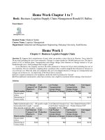
documents tips home work chapter 1 2 3 4 5 6 7 business logisticssupply chain management ronald h ballou

Home Work Chapter 1 to 7
Book: Business Logistics/Supply Chain Management Ronald H. Ballou
Excel sheet:

Logistics
management.xlsx

Student Name: Shaheen Sardar
Course Name: Logistics Management
Department: Industrial and Management Engineering, Hanyang University, South Korea.

Home Work 1
Chapter 1: Business Logistics/Supply Chain
Question 12: Suppose that a manufacturer of men's shirts can produce a dress shirt in its Houston, Texas, plant for
$8 per shirt (including the cost of raw materials). Chicago is a major market for 100,000 shirts per year. The shirt is
priced at $15 at Houston plant. Transportation and storage charges from Houston to Chicago amount to $5 per
hundredweight (cwt.). Each packaged shirt weighs 1 pound.
As an alternative, the company can have the shirts produced in Taiwan for $4 per shirt (including the cost of raw
materials). The raw materials, weighing about 1 pound per shirt, would be shipped from Houston to Taiwan at a cost
of $2 per cwt. When the shirts are completed, they are to be shipped directly to Chicago at a transportation and
storage cost of $6 per cwt. An import duty of $0.50 per shirt is assessed.
(a) From a logistics-production cost standpoint, should the shirts be produced in Taiwan?
(b) What additional considerations, other than economic ones, might be considered before making a final decision?
Solution:
cwt Material
Unit
Transport Cost Production
(Houston to
Cost
Plant Location Taiwan)
Houston plant

NO
$8
(USA)
Outsourcing to
$2
$4
Taiwan (Asia)

cwt Product
Transportation/
storage charges
(Houston to Chicago)
$5

Note: hundredweight (cwt) = 100 pounds weight
Each packed shirt weight = 1 pound
Raw material weight per shirt = 1 pound
Unit Material
Unit
Transport Cost Production
(Houston to
Cost
Plant Location Taiwan)
Houston plant
NO
$8
(USA)
Outsourcing to
$0.02
$4

Taiwan (Asia)

Unit Material Transport Cost = Raw Material Density/CWT
Unit Product Transport Cost = Product Density/CWT
Example: $2/100 = $0.02
Unit Product
Unit Product
Unit Import
Transportation/
Transportation
Duty
storage charges
/storage charges
(Houston to Chicago) (Taiwan to Chicago)
$0.05
NO
NO

NO

NO

cwt Product
Unit Import
Transportation
Duty
/storage charges
(Taiwan to Chicago)
NO
NO

$6

$0.06

$0.50

$0.50


Following formulas are used.
• Total Material Transport Cost = Product Volume * Unit Material Transport Cost
• Total Product Transport Cost = Product Volume* Unit Product Transport Cost
• Total Production Cost = Product Volume * Unit Production Cost
• Total Import Duty = Product Volume * Unit Import Duty
• Total Cost = Total Material Transport Cost + Total Product Transport Cost + Total Production Cost + Total
Import Duty
• Total Price = Product Volume * Shirt Price/unit
• Total Profit = Total Price - Total Cost
Total
Unit
Total
Total
Shirt
Product
Material
Product
Total
Production
Import
price/ Total price Profit

Volume
Transport Transport
Cost
Cost
Duty
unit
Plant Location
Cost
Cost
Houston plant
100000 $800,000
0
$5,000
0 $805,000 $15 $1,500,000 $695,000
(USA)
Outsourcing to
100000 $400,000
$2,000
$6,000 $50,000 $458,000 $15 $1,500,000 $1,042,000
Taiwan (Asia)
From a logistics-production cost standpoint, the shirts should be produced in Taiwan. There is a cost for raw
materials from Houston to Taiwan, but still is cheaper than the Houston plant when other costs are combined.
Following additional considerations might be considered before making a final decision.
• How long the shirts would be stored (holding cost) from plant-to-truck-to-final destination.
• Order processing cost for suppliers needs to be done strategically (to have least cost of shipping to Chicago).
• How order is transported at least cost, most efficiently, and within the time allotted.
• Supplier availability in Taiwan.
• Capacity availability in Taiwan.
• Risk of late delivery in Taiwan.
• Quality and reliability issues in Taiwan.

• Effective inventory lot-sizing in Taiwan.
• Other strategic considerations in USA as well as in Taiwan.

Home Work 2
Chapter 2: Logistics/Supply Chain Strategy and Planning
Question 13: The traffic manager of the Monarch Electric Company has just received a rate reduction offer from a
trucking company for the shipment of fractional horsepower motors to the company's field warehouse. The proposal
is a rate of $3 per hundredweight (cwt.) if a minimum of 40,000 pounds is moved in each shipment. Currently,
shipments of 20,000 pounds or more are moved at a rate of $5 per cwt. If the shipment size falls below 20000
pounds, a rate of $9 per cwt. applies.
To help the traffic manager make a decision, the following information has been gathered:

Annual demand on warehouse

5,000 motors a year


Warehouse replenishment orders

43 orders a year

Weight of each motor, crated

175 lb per motor

Standard cost of motor in warehouse

$200 per motor

Stock replenishment order handling cost

$15 per order

Inventory carrying cost as percentage of average value of inventory on hand for a year
Handling cost at warehouse

$ 0.30 per cwt.

Warehouse space

unlimited

25% per year

Should the company implement the new rate?

Solution:
Circumstance 1: Rate for shipment weight ≥ 40000 = $3 per cwt. (New proposal)
Circumstance 2: Rate for shipment weight ≥ 20000 = $5 per cwt. (Present)
Circumstance 3: Rate for shipment weight < 20000 = $9 per cwt. (Present)
Shipment size is more than 20000 or minimum 40000, so we will not investigate Circumstance 3.
Weight of total motors (annual requirement) = 5000 motors/year * 175 lb. /motor = 875000 lb. / year = 8750
cwt/year (i.e. 1 cwt = 100 lb.)
Cost for Circumstance 1: (For new proposal)
Trucking cost = $3/cwt * 8750 cwt / year = $ 26250/year

Ordering cost = 21 orders * $ 15 /order = $ 315

Handling cost at warehouse = $0.3/cwt *8750 cwt / year = $ 2625
Total Cost = $ 26250 + $ 315 + $ 5715 + $ 2625 = $ 34905

Cost for Circumstance 2: (For present situation)
Trucking cost = $5/cwt * 8750 cwt / year = $ 43750

Ordering cost = 43 orders * $ 15 /order = $ 645

Handling cost at warehouse = $0.3/cwt *8750 cwt/ year = $ 2625


Total Cost = $ 43750 + $ 645 + $ 2857 + $ 2625 = 49877
Circumstance 1 Total Cost: (For new proposal) = $ 34905
Circumstance 2 Total Cost: (For present situation) = $ 49877

Yes, the company should implement the new rate.

Home Work 3
Chapter 3: Logistics/Supply Chain Product
Question 11: Davis Steel Distributors is planning to set up an additional warehouse in its distribution network.
Analysis of item-sales data in its other warehouses shows that 25% of the items represent 75% of the sales volume.
The company also has an inventory policy that varies with the items in the warehouse. That is, the first 20% of the
items are the A items and are to be stocked with turnover ratio of 8. The next 30% of the items, or B items, are to
have turnover ratio of 6. The remaining C items are to have a turnover ratio of 4. There are to be 20 products held at
the warehouse with sales forecasted to be $2.6 million annually. What dollar value of the average inventory would
you estimate for the warehouse?
Solution:

Number of items = N = 20
Sales = $2.6 million = $2600000

Cumulative sales proportion is

Projected items sales = difference between cumulative sales for successive items


Alternative Method
Cumulative sales proportion is

Cumulative sales () =$2600000* = 1,800,000
Projected Item Sales () = $1,800,000

Cumulative sales () =$2,600,000* = $2,340,000
The product group B sales will be A+B sales less A sales
Projected Item Sales () = = $2,340,000- $1,800,000 = $540,000


Cumulative sales () =$2,600,000* = 2,600,000
The product group C sales will be A+B+C sales less A+B sales
Projected Item Sales () = = 2,600,000-$2,340,000= $260,000

Dollar value of the average inventory for the warehouse is

Question 12: Beta Products is planning to add another warehouse. Ten products from the entire line are to be stored
in the new warehouse. These products will be the A and B items. All C items are to be served out of the plant.
Forecasts of annual sales that are expected in the region of the new facility are 3 million cases (A, B, and C items).
Historical data show that 30 percent of the items account for 70 percent of the sales. The first 20 percent of the entire
line are designated as A items, the next 30 percent as B items, and the remaining 50% as C items. Inventory turnover
ratios in the new warehouse are projected to be 9 for A items and 5 for B items. Each inventory item, on the average,
requires 1.5 cubic feet of space. Product is stacked 16 feet high in the warehouse.
What effective storage space is needed in square feet excluding aisle, office, and other space requirements?
Solution:
All C items are to be served out of the plant. So, we will consider only A and B.

Number of items = N = 10
Sales = $3 million = $3000000

Cumulative sales proportion is

Projected items sales = difference between cumulative sales for successive items


Space requirement = 1.5 cubic feet
Stack height requirement = 16 feet

Effective storage space required = 33110
Question 13: An analysis of the product line items in the retail stores of the Save-More Drug chain shows that 20%
of the items stocked account for 65% of the dollar sales. A typical store carries 5,000 items. The items accounting
for the top 75% of the sales are replenished from warehouse stocks. The remainder is shipped directly to stores from
manufacturers or jobbers. How many items are represented in the top 75% of sales?
Solution:

From equation (1), we have

Now

From equation (2), we have


29% of the items represent the top 75% of sales
Total number of items = 5,000
Number of items that represent 75% of sales = 0.29*5000 = 1450
Question 14: The cost associated with producing, distributing, and selling a domestically produced automotive

component to Honda in Japan can be summarized as follows:
Cost type
Purchased materials
Manufacturing labor
Overhead
Transportation
Sales
Profit

Cost per Unit, $
25
10
5
Varies by shipment size
8
5

Transportation costs vary as follows. If the purchase (shipping) quantity is 1000 units or less, the
transportation cost is $5 per unit. For more than 1000 units but less than or equal to 2000 units, the transportation
cost is $4 per unit. For more than 2000 units, the transportation cost is $3 per unit.
Construct a price schedule, assuming the vendor would like to pass the transportation economies on to the
customer. Indicate the discount percentage the customer will receive through buying at various quantities.
Solution:
Case 1: Quantity is 1000 units or less
Total cost = $25 + $10 +$5 + $5 + $8 + $5 = $58
Case 2: Quantity is more than 1000 units but less than or equal to 2000 units
Total cost = $25 + $10 +$5 + $4 + $8 + $5 = $57
Discount rate between Case 1 and Case 2:

Case 3: Quantity is more than 2000 units

Total cost = $25 + $10 +$5 + $3+ $8 + $5 = $56
Discount rate between Case 1 and Case 3:

Discount rate between Case 2 and Case 3:

Home Work 4
Chapter 4: Logistics/Supply Chain Customer Service


Question 6: The Cleanco Chemical Company sells cleaning compounds (dishwashing powders, floor cleaners,
nonpetroleum lubricants) in a keenly competitive environment to restaurants, hospitals and schools. Delivery time
on orders determines whether a sale can be made. The distribution system can be designed to provide different
average levels of delivery time through the number and location of warehousing points, stocking levels and order
processing procedures. The psychical distribution manager has made the following estimates of how service affects
sales and the cost of providing service levels:

Estimated annual sales (millions of $)
Cost of distribution (millions of $)

Percentage of orders delivered in one day
60
70
80
90
95
8.0
10.0
11.0
11.5
11.8

6.0
6.5
7.0
8.1
9.0

50
4.0
5.8

100
12.0
14.0

(a) What level of service should the company offer?
(b) What effect would competition likely have on the service level decision?
Solution (a): Profit = Estimated annual sales – cost of distribution

Estimated annual sales (millions of $)
Cost of distribution (millions of $)

50
4.0
5.8

Profit (millions of $)

-1.8

Percentage of orders delivered in one day

60
70
80
90
95
8.0
10.0
11.0
11.5
11.8
6
6.5
7
8.1
9
2

3.5

4

3.4

2.8

100
12.0
14
-2

Profit is $4 million at 80% service level. Company maximizes the profit when it serves at 80% service level.
Company should offer 80% of service level.
Solution (b): Suppose the product’s price and quality is the same in all competing companies. If a company A
increases its service level, other competitor companies will also increase their service levels. Based on competition,
the company A will change its service level, resulting in change in its profit (otherwise loss of customers).
Question 7: Five years ago, Norton Valves, Inc., introduced and publicized a program under which 56 items in its
hydraulic valve line would be made available on a 24-hour-delievery basis, instead of normal 1-to 12-week delivery
period. Quick order processing, stocking to anticipated demand, and using premium transportation services when
necessary were elements of the 24-hour delivery program. Sales history was recorded for the five years before the
service change as well as for a five-year period after the change. Because only a portion of the product family was
subject to the service improvement, the remaining products (102 items) served as a control group. Statistics for one
of the test product groups showing the before and after annual units sales levels are given as follows:
Sales before service change
Sales after service change
5-Year Average
Standard
5-Year Average
Standard Deviation
Deviation
Test group
1342
335
2295
576
Control group
185
61
224
76
 Standard Deviation: For the individual sales

 Test group: Products in family with 24-hour delivery
 Control group: Products in family with 1-to 12-week delivery
Product Family

The average value of products in this family was $95 per unit. The incremental cost for the improved service was $2
per unit, but the company did not intend to pass along the costs as a price increase. Instead it hoped that additional
sales volume would more than offset the added costs. The profit margin on sales at the time was 40 percent.
(a) Should the company continue the premium service policy?
(b) Appraise the methodology as a way of accuracy determining the sales-service effect.


Solution: (a)
• Before: (1342+185)*95*0.40 = $58026
• After: (2295+224)*95*0.40 – (2295*2) = $91132
• Company should continue the premium service policy.
Solution: (b) We appraise the methodology as a way of accurately determining the sales-service effect.
Question 8: A food company is attempting to set the customer service level (in-stock probability in its warehouse)
for a particular product line item. Annual sales for the item are 100,000 boxes, or 3846 boxes biweekly. The product
cost in inventory is $10, to which $1 is added as profit margin. Stock replenishment is every two weeks, and the
demand during this time is assumed to be normally distributed with a standard deviation of 400 boxes. Inventory
carrying costs are 30% per year of item value. Management estimates that a 0.15% change in total revenue would
occur for each 1% change in the in-stock probability.
(a) Based on this information, find the optimum in-stock probability for the item.
(b) What is the weakest link in this methodology? Why?
Solution: (a) Optimum service level is the point where the change of cost equals to the change of profit (∆p = ∆c)
∆p = Trading margin*sales response rate *annual sales
∆p = $1*0.0015*100000
∆p = $150 per year (per 1% change in the service level)
∆c = annual carrying cost * standard product cost * ∆z*demand standard deviation over replenishment lead time
∆c = 0.30*$10*∆z*400

∆c = $ 1200 ∆z
∆p = ∆c
$150 = $1200*$∆z

For the change in z found in a normal distribution table, the optimum in-stock probability during the lead time is
about 96-97%.
Solution: (b) The weakest link in methodology is that ∆p is assumed as constant for all service levels, in fact, in
most cases ∆p is a decreasing function of service level. We do not have the correct data about interrelation of service
level and sales. (Weakest link in this analysis is estimating the effect that a change in service will have on revenue).
Question 9: An item in the product line for the food company discussed in question 8 has the following
characteristics:
Sales response rate = 0.15% change in revenue for a 1% change in the service level
Trading margin = $0.75 per case
Annual sales through the warehouse = 80,000 cases
Annual carrying cost = 25 %
Standard product cost = $10
Demand standard deviation = 500 cases per 1 week lead time
Lead time = 1 week
Find the optimum service level for this item.


Solution: Optimum service level is the point where the change of cost equals to the change of profit (∆p = ∆c)
∆p = Trading margin*sales response rate *annual sales
∆p = $0.75*0.0015*80000
∆p = $90 per year (per 1% change in the service level)
∆c = annual carrying cost * standard product cost *∆z*demand standard deviation over replenishment lead time
∆c = 0.25*$10*∆z*500
∆c = $ 1250 ∆z
∆p = ∆c
$90 = $1250*∆z

For the change in z found in a normal distribution table, the optimum service level for this item is about 92-93%.
Question 10: A retailer has targeted a shelf item to be out of stock only 5% of the time ( m). Customers have come
to expect this level of product availability, so much so, that when the out of stock percentage increases, customer
seek substitutes and lost sales occur. From market research studies, the retailer has determined that when the out of
stock probability increases to the 10% level (y), sales and profit drop to one-half of those at target level. Decreasing
the out of stock percentage from the target level seems to have little impact on sales, but it does increase inventory
carrying cost substantially. The following data have been collected on the item:
Price
Cost of item
Other expenses associated with stocking the item
Annual item sold @ 95% in-stock

$5.95
4.25
@0.30
880

The retailer estimates that every one percentage point that the in-stock probability is allowed to vary from the target
level, the unit cost of supplying the item decreases according to C = (1.00-0.10) (i.e. y-m), where C is the cost per
unit, y is the out-of-stock percentage, and m is the target out-of-stock percentage
How much variability from the target stocking percentage should the retailer allow?
Solution:

The retailer should not allow the out of stock percentage to deviate more than 1.79% and should not allow the out of
stock level to fall below 1.79 + 5 = 6.79%.


Home Work 5
Chapter 5: Order Processing and Information Systems

Question 5: A logistics manager for a television producer in South Korea has been given the responsibility for
setting up a logistics information system for his company. How would you answer his question below?
(a) What types of information do I want from the information system? Where would I obtain the information?
(b) Which item in information database should I retain in the computer for easy access? How should I handle the
remainder?
(c) What types of decision problems would the information system help me address?
(d) What models for data analysis would be most useful in dealing with these problems?
Answer (a): We can get amount of sales, times, sales location, order data, inventory rate, transport cost, etc. from
customers, company, books, and company files.
Answer (b): Logistics manager decides the criteria for judgment when he makes the decision. For example:
 How important is the data stored on computer database?
 What data is not required to keep on computer due to computer memory problems?
 Is it necessary to respond quickly?
 How frequent efforts are required for data management?
Answer (c): Information system helps the company to solve logistics problems.
Answer (d): Mathematical and statistical models.
Question 6: For the following companies, suggest the types of data that should be collected to plan and control their
supply chain:
(a) A hospital
(b) A city government
(c) A tire manufacturer
(d) A retailer of general merchandise
(e) An ore-mining company
Answer (a): A hospital = Number of customers, rooms, patients, doctors, etc.
Answer (b): A city government = Number of customers, employees, etc.
Answer (c): A tire manufacturer = Number of orders, sales, location, etc.
Answer (d): A retailer of general merchandise = Information of items, inventory, etc.
Answer (e): An ore-mining company = Expected demand, logistics, amount of minerals, etc.

Home Work 6

Chapter 6: Transport Fundamentals

Question 14: A power company in Missouri can buy coal for its generating plants from western mines in
Utah or from eastern mines in Pennsylvania. The maximum purchase price for coal of $20 per ton at the Missouri
plant is set according to the price of competing energy forms. The cost to mine coal in the West is $17 per ton and
in the East is $15 per ton. Transportation cost from the eastern mines is $3 per ton. What is the value of
transportation from the western mines?
Solution:
The cost to mine coal + transportation cost should be ≤ $20 per ton.
For East:
Cost to mine coal in the East = $15
Transportation cost in the East = $3


Total cost in the East = $15 + $3 = $18
For West:
Cost to mine coal in the West = $17
Transportation cost in the West = $x
Total cost in the West = $17 + $x
The maximum purchase price for coal is decided by competition.
Now, total cost in the West must be as follow:
$17 + $x ≤ $18
Transportation cost in the West must be as follow:
$x ≤ $18 - $17
$x ≤ $1
Therefore, Transportation cost in the West must be ≤ $1, if we want to purchase coal from West.

Question 15: Shipments for a certain product originate at point X and are to be sent to points Y and Z. Y is
an intermediate point to X and Z. The rate of Y is $1.20 per cwt., but due to competitive condition at Z, the rate of Z
is $1.00 per cwt. (hundredweight). Apply the principle of blanketing back, and explain how it eliminates rate

discrimination.
Solution:
Blanketing is a form of rate discrimination, but the benefits of rate simplification for both carriers and shippers
outweigh the disadvantages.
X----------------Y--------------------Z
X to Y = $1.20
Y to Z = $1.00
Cost 1
Cost 2
If competitive conditions do not permit an increase in the rate to Z, then all rates that exceed $1 per cwt. on a line
between X and Z should not exceed $1 per cwt. Therefore, the rate to Z is blanketed back to Y so that the rate to Y is
$1 per cwt. By blanketing the rate to Z on intervening points, no intervening point is discriminated against in terms
of rates.

Question 16: Using Table 6-4, 6-5, and 6-6, determine the freight charges for the following shipments:
a) A 2500-lb shipment of paper place mats with printed advertising moving from New York to Los Angeles.
b) A 150-lb shipment of rubber displays for advertising purposes moving from New York to Providence, RI.
c) A 27000-lb shipment of emery cloth in packages moving from Louisville, Kentucky, to Chicago, Illinois. Note:
For any product classification number below 50, use 50 in Table 6-6.
d) A 30000-lb shipment of cat accessories at a density of 10 lb. per cubic foot moving between Louisville,
Kentucky, and Chicago, Illinois.
e) A 24000-lb shipment of advertising circulars not printed on newsprint moving between Louisville, Kentucky, and
Chicago, Illinois. A rate discount of 40 percent is offered.
Solution (a): From Table 6-4, the item number for place mats is 4745-00. Classification is 100, and minimum
weight is 20000 lb. The 2500 lb. is less than minimum weight of 20000 lb. for a truckload shipment. From the Table
6-5, for Los Angeles, the rate for shipment of ≥ 20000 is 87.27 cents/cwt. The shipping charges are as follows:
25 cwt * $87.27 = $2181.75
Solution (b): From Table 6-4, the item number for rubber displays for advertising purposes is 4980-00.
Classification is 100, and minimum weight is 20000 lb. The 150 lb. is less than minimum weight of 20000 lb. for a

truckload shipment. From the Table 6-5, for Providence, RI, the rate for minimum shipment is 93.51 cents/cwt. The
shipping charges are as follows:
1.5cwt * $93.51 = $140.265
The rate for < 500 lb. is 54.01 cents/cwt. The shipping charges using the < 500 lb. are as follows:
$54.01 * 1.5 cwt = $81.02
$81.02 is less than $140.265. We should pay the minimum charges.
Solution (c): From Table 6-4, the item number for emery cloth in packages is 2055-00. Classification is 55 for Less
Than Truckload (LTL), and 37.5 for Truckload. Minimum weight is 36000 lb. There are following three options
(Using Table 6-6):
• Ship LTL at class 55 and 27000 lb. shipment. ($5.65/cwt*270 = $1525.50)
• Ship at class 55 and 30000 lb. rate. ($3.87/cwt*300 = $1161) = Lowest cost
• Ship at class 37.5 and 36000 lb. rate. ($3.70/cwt*360 = $1332.50)
Solution (d): From Table 6-4, the item number for cat accessories is 2070-00. Classification is 65 (see 2070-07: 10
but less than 12). Using Table 6-6, the rate at 30000 lb. is $4.21/cwt, and shipping charges are as follows:
4.21*300 = $1263
Solution (e): Using Table 6-4, not printed on newsprint are classified 55 (4860-00) for a Truck load of 24000 lb.
Calculate break weight as follows.

Since current shipping weight of 24000 lb. exceeds the break weight, ship as if 30000 lb. Hence,
3.87*300 = $1161. Now, discount the charges by 40 percent as follows:
$1161 * (1-0.40) = $696.60

Question 21:

A traffic manager has two options in scheduling a truck to make multiple pickups and
deliveries. The pick-up delivery problem is shown pictorially in Figure 6-11. The traffic manager can ship the
accumulated volumes as single shipments between the designated points or can use the stop-off privilege at $25 per
stop for any or all portions of the trip. If the traffic manager wishes to minimize shipping costs, which alternative
should be chosen? Assume that the final destination point incurs the stop-off change?

Solution:

In Figure 6.11, there are two stops (i.e. A and B) where we can load the total 40,000 lb. quantity in such a way that:
• A = (25000 lb. for C and D)


•

B = (15000 lb. for C)

In Figure 6.11, there are two stops (i.e. C and D) where we can deliver the total 40,000 lb. quantity in such a way
that:
• C = (18000 lb. from A or B)
• D = (22000 lb. from A)
According to Figure 6.11, alternative 1 is without stop-off.

Alternative 1: Separate shipment (without stop-off privilege)
Loading/unloading

Route

Rate $/cwt.

22000
3000 (i.e. 25000-22000)
15000

A→D
A→C
B→C

$3.20
$2.50
$1.50

cwt Rate
Stop-off
$/cwt.
charge
$0.032
$0.025
$0.015
Total charges

Charges
$704
$75
$225
$1,004

Alternative 2: With stop-off privilege
Loading/unloading

Route

Rate $/cwt.

25000
40000 (i.e. 25000+15000)
Stop-off @ C

Stop-off @ D

A→B
B→D

$1.20
$2.20

cwt Rate
$/cwt.
$0.012
$0.022

Stop-off
charge
$25
$25
Total charges

-

-

-

-

Charges
$300
$880

$25
$25
$1,230

Alternative 3: With stop-off privilege
Loading/unloading

Route

Rate $/cwt.

40000
Stop-off @ B
Stop-off @ C
Stop-off @ D

A→D

$3.20

cwt Rate
$/cwt.
$0.032

Stop-off
charge
$25
$25
$25
Total charges

-

-

-

-

Charges
$1,280
$25
$25
$25
$1,355

Various other alternatives can be checked. In the present cases, there appears to be no advantage of stop-off
privilege.

Home Work 7
Chapter 7: Transport Decisions
Question 1: The Wagner Company supplies electric motors to Electronic Distributors, Inc.on a delivered-price
basis. Wagner has the responsibility for providing transportation. The traffic manager has three transportation service
choices for delivery----rail, piggyback, and truck. He has compiled the following information.
Transport Mode
Rail

Transit Time, Days
16

Rate, $/Unit
25.00

Shipment Size, Units
10,000


Piggyback
Truck

10
4

44.00
88.00

7,000
5,000

Electronic Distributors purchases 50,000 units per year at a delivered contract price of $500 per unit. Inventorycarrying cost for both companies is 25 percent per year. Which mode of transportation should Wagner select?
Solution:
Selecting a mode of transportation requires balancing the direct cost of transportation with the indirect costs of both
vendor and buyer inventories plus the in-transit inventory costs. The differences in transport mode performance
affect these inventory levels, and, therefore, the costs for maintaining them, as well as affect the time that the goods
are in transit. We wish to compare these four cost factors for each mode choice.

We use following formulas:

• Transport cost = transportation rate * annual demand
• Item value at buyer's inventory = price per unit

• Item value at vendor's inventory = price per unit – transport cost per unit (e.g. 500– 25 = 475 for rail)
• In-transit inventory cost= Inventory carrying cost * item value at vendor's inventory* annual demand *
(time in transit /365)

• Inventory cost of Wagner (supplier) = Inventory carrying cost * item value at vendor's inventory*
(shipping quantity/2)

• Inventory cost of Electronic Distributors (Buyer) = Inventory carrying cost * item value at buyer's inventory*
(Shipping quantity /2)

Transportation rate
Shipping quantity, units
Transit Time, Days

Rail
25
10000
16

Transport cost
1250000
In-transit inventory cost
260274
Inventory cost of Wagner (supplier)
593750
Inventory cost of Electronic Distributors (Buyer)
625000
Total Cost 2729024
Mode of transportation
Rail

Piggyback
44
7000
10

truck
88
5000
4

2200000
156164
399000
437500
3192664
Piggyback

4400000
56438
257500
312500
5026438
truck

Rail has the lowest total cost.


Question 2: Suppose two truck services are being considered for deliveries from a company plant to one of its
warehouses. Service B is cheaper but slower and less reliable than service A. The following information has been

assembled:
Demand (known)
Order cost
Production price, f.o.b. source
Shipping quantity
In-transit carrying cost
Inventory carrying cost
In-stock probability during the lead time
Out-of-stock costs
Selling days

Transit time (LT)
Variability (std. dev., sLT)
Rate

Service A
4 days
1.5 days
$12.00/cwt

9600 cwt./year
$100/order
$50/cwt
As per EOQ
20%/year
30%/year
30%
Unknown
365 days/year
Service B

5 days
1.8 days
$11.80/cwt

A reorder point control method of inventory control is used at the warehouse. From the point of view of the
inventory in the warehouse, which truck service should be selected? (Note: Refer to Chapter 9 on inventory
management for discussion of the reorder point method of inventory control. Hint: The standard deviation of the
demand-during-lead-time distribution is s’ = d(sLT), where sLT is assumed the transit time variability and d is the daily
demand rate.)
Solution:
As in question 1, this problem is one of balancing transport costs with the indirect costs associated with inventories.
However, in this case we must account for the variability in transit time as it affects the warehouse inventories. We
can develop the following decision table.


Now, we use following formulas:

• Transport cost = transportation rate * annual demand
• In-transit inventory cost = Inventory carrying cost * Production price * annual demand * (time in transit/365)
• Inventory cost of Plant = In-transit carrying cost * Production price * (shipping quantity for plant/2)
• Inventory cost of Warehouse = Inventory carrying cost * Production price * (Shipping quantity /2) + Inventory
carrying cost * Production price * Safety stock (r).
Annual demand
Inventory-carrying cost
Production price
In-transit carrying cost
Shipping quantity for plant

Transportation rate
Shipping quantity, units

Transit Time, Days
Safety stock (r)
Transport cost
In-transit inventory cost
Inventory cost of Plant
Inventory cost of Warehouse
Total Cost

9600
0.30
50
0.20
357.8
A
12
321.3
4
50.5

B
11.8
321.8
5
60.6

115200
1052
2684
3927
122863

113280
1315
2684
4107
121385

Service B appears to be less expensive.

Question 3: The Transcontinental Trucking Company wishes to route a shipment from Buffalo to Duluth over
major highways. Because time and distance are closely related, the company dispatcher would like to find the
shortest route. A schematic network of the major highway links and mileage between city pairs is shown below (i.e.
Figure 7-20 in Book). Find the shortest route through the network by using the shortest route method.


Solution:
Using the shortest route method, results are show in table below. The shortest route is defined by tracing the links
from the destination node. They are shown as A→D → F→ G for a total distance of 980 miles.

Question 4: The U.S. Army Materiel Command was preparing final arrangements to move its M113 FullTracked Armored Personnel Carrier from various subcontractors’ manufacturing facilities to intermediate storage
facilities at Letterkenny, Pennsylvania, for those units destined for Europe and for several army bases within the
United States. The production schedule for December plus the units on hand at the plant and requirements for
December are shown as follows:
Production schedule for December
Cleveland, OH
South Charleston, WV
San Jose, CA

150 units plus 250
150

150


Requirements for December
U.S. Army, Europe via Letterkenny, PA
Fort Hood, TX
Fort Riley, KS
Fort Carson, CO
Fort Benning, GA

300 units
100
100
100
100

Figure 7-21 (see Book) shows the location of the supply and demand points as well as the per-unit transportation
costs from supply to demand points. Find the least-costly delivery plan for December to meet the requirements, but
do not exceed the production schedule requirements.
Solution:
In this actual problem, the U.S. Army used the transportation method of linear programming to solve its allocation
problem. The problem can be set up in matrix form as follows:

The cell values shown in bold represent the number of personnel carriers to be moved between origin and
destination points for minimum transportation costs of $153,750. An alternative solution at the same cost would be
as follows:

Question 5:

The Evansville Local School District provides bus transportation for its elementary

schoolchildren. One bus has been assigned to the neighborhood, as defined in Figure 7-22 (see Book). Each year
there is a new roster of children, and the location of the stops for them can be plotted on a map. Sequencing the stops
determines the time and distance required to complete the bus tour. Using your best cognitive skills, design the
shortest bus tour possible given the following conditions:
• Only one bus is to be used.
• The bus starts at the elementary school and returns to it.
• Each stop is to be visited.
• Children may be picked up or dropped off from either side of the street.
• A pickup or dropoff at a corner may be made from either adjacent street.


•
•

No U-turns are permitted.
The bus has adequate capacity to transport all the children on the route.

Use a ruler or linear grid to determine the total distance for the bus tour.
Solution:
This problem can be used effectively as an in-class exercise. Although the problem might be solved using a
combination of the shortest route method to find the optimum path between stops and then a traveling salesman
method to sequence the stops, it is intended that students will use their cognitive skills to find a good solution. The
class should be divided into teams and given a limited amount of time to find a solution. They should be provided
with a transparency of the map and asked to draw their solution on it. The instructor can then show the class each
solution with the total distance achieved. From the least-distance solutions, the instructor may ask the teams to
explain the logic of their solution process. Finally, the instructor may explore with the class how this and similar
problems might be treated with the aid of a computer. Although the question asks the student to use cognitive skills
to find a good route, a route can be found with the aid of the ROUTER software in LOGWARE. The general
approach is to first find the route in ROUTER without regard to the rectilinear distances of the road network.
Because this may produce an infeasible solution, specific travel distance are added to the database to represent

actual distances traveled or to block infeasible paths from occurring. A reasonable routing plan is shown in the
Figure below:

The total distance for the route is 9.05 miles and at a speed of 20 miles per hour, the route time is approximately 30
minutes. The ROUTER database that generates it is given below.



Question 6:

Dan Pupp is a jewelry salesperson who calls on store accounts in the Midwest. One of his
territories is shown in Figure 7-23 (see Book). His mode of operation is to arrive at the territory the night before
making his calls to stay at one of the local motels. He covers the region in two days and leaves the morning of the
third day. Since he pays his own expenses, he would like to minimize his total costs for serving the accounts.
Accounts 1 to 9 are covered the first day, and the remainder are visited the second day. He would like to compare
two strategies:
Strategy 1: Stay at Motel M2 all three nights at $49.00 per night.
Strategy 2: Stay at Motel M1 to visit accounts 1 to 9, staying there two nights at $40.00 per night. Then, stay at
Motel M3 one night at $45.00 per night to visit accounts 10 to 18. After visiting accounts 1 to 9, he returns to M 1 to
stay overnight before moving to M 3. He then stays overnight at M 3 before moving on the next morning. The distance
between M1 and M3 is 36 miles.
Disregard any distance that he travels to and from the territory. Dan figures mileage costs at $0.30 per mile.
Which strategy seems best for Dan?
Solution:
Strategy 1 is to stay at motel M 2 and serve the two routes on separate days. Using the ROUTESEQ module in
LOGWARE gives us the sequence of stops and the coordinate distance. The routes originating at M 2 would be as
follows:


Question 7: A bakery delivers daily to five large retail stores in a defined territory. The driver person for the

bakery loads goods at the bakery, makes deliveries to the retail stores, and returns to the bakery. A diagram for the
territory is shown in Figure 7-24 (see Book). The associated network travel times in minutes are:
To 
Bakery
1
2
From
3
4
5

Bakery
0
22
47
39
57
21

1
24
0
35
27
42
16

2
50
32

0
17
18
57

3
38
23
15
0
16
21

4
55
45
21
14
0
41

5
20
18
60
25
42
0

(a) What is the best routing sequence for the delivery truck?

(b) If loading or unloading times are significant, how might they be included in the analysis?
(c) Retail store 3 is located in such a densely populated urban area that the travel times to and from this point may
increase by as much as 50 percent, depending on the time of the day. Travel times for other points remain relatively
unchanged. Would the solution in part (a) be sensitive to such variations?
Solution:
(a) Since distances are asymmetrical, we cannot use the geographically based traveling salesman method in
LOGWARE. Rather, we use a similar module in STORM that allows such asymmetrical matrices, or the problem is
small enough to be solved by inspection. For this problem, the minimal cost stop sequence would be as follows:
Bakery →Stop 5 → Stop 3→ Stop 4→ Stop 2→Stop 1→Bakery (with a tour time of 130 minutes)
(b) Loading/unloading times may be added to the travel times to a stop. Problem may then be solved as in part a.
(c) Travel times between stop 3 and all other nodes are increased by 50 percent. Remaining times are left unchanged.
Optimizing on this matrix shows no change in the stop sequence. However, tour time increases to 147.50 minutes.


Question 8:

Sima Donuts supplies its retail outlets with the ingredients for making fresh donuts. A central
warehouse from which trucks are dispatched is located in Atlanta. Trucks can leave the Atlanta warehouse as early
as 3 A.M. to make pallet-load deliveries to the Florida market and make returns at any time. The trucks may also
pick up empty containers and supplies from vendors in the general area. Pickups are allowed only after all deliveries
on a route are made. A simple linear grid is placed over the Georgia-Florida area and grid coordinates found for
warehouse, retail, and vendor sites. The 0, 0 coordinates are in the northeast corner. For example, the Atlanta
warehouse is located at X = 2084, Y = 7260. The scaling factor on the map, including a road circuitry factor, is
0.363. The total time on a route may be 40 hours and total route distance may be up to 1400 miles. Team drivers are
used so that no overnight breaks are required, but one-hour rest breaks are allowed at 12-noon and 8 P.M. each day.
Average driving speed is taken to be 45 miles per hour. Additional data about the stops are as follows:
No
1
2
3

4
5
6
7
8
9
10
11

Stop location
Tampa, FL
Clearwater, FL
Daytona Beach, FL
Fort Lauderdale, FL
North Miami, FL
Oakland Park, FL
Orlando, FL
St Petersburg, FL
Tallahassee, FL
West Palm Beach, FL
Miami-Puerto Rico

Stop
Volume,
XYLoading/ Unloading
type
Pallets Coordinate Coordinate
Time (Min.)
Delivery
20

1147
8197
15
Pickup
14
1206
8203
45
Delivery
18
1052
7791
45
Delivery
3
557
8282
45
Delivery
5
527
8341
45
Pickup
4
565
8273
45
Delivery
3

1031
7954
45
Pickup
3
1159
8224
45
Delivery
3
1716
7877
45
Delivery
3
607
8166
45
Delivery
4
527
8351
45
Total 80

Time Windows
Open
Close
6:00 A.M. 12:00 A.M.a
6:00 A.M. 12:00 A.M.

6:00 A.M. 12:00 A.M.
3:00 A.M. 12:00 A.M.
6:00 A.M. 12:00 A.M.
3:00 A.M. 12:00 A.M.
3:00 A.M. 12:00 A.M.
3:00 A.M. 12:00 A.M.
10:00 A.M. 12:00 A.M.
6:00 A.M. 12:00 A.M.
6:00 A.M. 12:00 A.M.

a

Midnight

There are three trucks with a 20-pallet capacity, one with a 25-pallet capacity, and one with a 30-pallet capacity. The
cost for drivers and truck is $1.30 per mile. Design the routes for this set of deliveries and pickups. Which trucks are
to be assigned to which routes? What is the dispatch plan? What is the cost for dispatch?
Solution:
This may be solved by using the ROUTER module in LOGWARE. The screen set up for this is as follows: