Orifices W. H. HOWE (1969) B. G. LIPTÁK (1995), REVIEWED BY S. RUDBÄCH
Bạn đang xem bản rút gọn của tài liệu. Xem và tải ngay bản đầy đủ của tài liệu tại đây (1.02 MB, 18 trang )
2.15
Orifices
W. H. HOWE (1969)
J. B. ARANT
FE
B. G. LIPTÁK (1995), REVIEWED BY S. RUDBÄCH
In Quick Change Fitting
(1982, 2003)
FO
FE
Flange Taps
Fixed Restriction
FE
FT
Vena Contracta Taps
or Radius Taps
Integral Orifice
Transmitter
Flow Sheet Symbol
Design Pressure
For plates, limited by readout device only; integral orifice transmitter to 1500 PSIG
(10.3 MPa)
Design Temperature
This is a function of associated readout system, only when the differential-pressure
unit must operate at the elevated temperature. For integral orifice transmitter, the
standard range is −20 to 250°F (−29 to 121°C).
Sizes
Maximum size is pipe size
Fluids
Liquids, vapors, and gases
Flow Range
From a few cubic centimeters per minute using integral orifice transmitters to any
maximum flow, limited only by pipe size
Materials of Construction
There is no limitation on plate materials. Integral orifice transmitter wetted parts can
be obtained in steel, stainless steel, Monel , nickel, and Hastelloy .
Inaccuracy
The orifice plate; if the bore diameter is correctly calculated, prepared, and installed,
the orifice can be accurate to ±0.25 to ±0.5% of actual flow. When a properly
calibrated conventional d/p cell is used to detect the orifice differential, it will add
±0.1 to ±0.3% of full-scale error. The error contribution of properly calibrated “smart”
d/p cells is only 0.1% of actual span.
Smart d/p Cells
Inaccuracy of ±0.1%, rangeability of 40:1, built-in PID algorithm
Rangeability
If one defines rangeability as the flow range within which the combined flow measurement error does not exceed ±1% of actual flow, then the rangeability of conventional orifice installations is about 3:1 maximum. When using intelligent transmitters
with automatic switching capability between the “high” and the “low” span, the
rangeability can approach 10:1.
Cost
A plate only is $100 to $300, depending on size and materials. For steel orifice flanges
from 2 to 12 in. (50 to 300 mm), the cost ranges from $250 to $1200. For flanged meter
runs in the same size range, the cost ranges from $500 to $3500. The cost of electronic
or pneumatic integral orifice transmitters is between $1500 and $2500. The cost of d/p
transmitters ranges from $1000 to $2500, depending on type and “intelligence.”
Partial List of Suppliers
ABB Process Automation (www.abb.com/processautomation) (incl. integral orifices)
Daniel Measurement and Control (www.danielind.com) (orifice plates and plate changers)
The Foxboro Co. (www.foxboro.com) (incl. integral orifices)
Honeywell Industrial Control (www.honeywell.com/acs/cp)
Meriam Instrument (www.meriam.com) (orifice plates)
Rosemount Inc. (www.rosemount.com)
Tri-Flow Inc. (www.triflow.com)
259
© 2003 by Béla Lipták
260
Flow Measurement
In addition, orifice plates, flanges and accessories can be
obtained from most major instrument manufacturers.
data, more accurate and versatile test and calibrating equipment, better differential-pressure sensors, and many others.
Theory of Head Meters
HEAD-TYPE FLOWMETERS
Head-type flowmeters compose a class of devices for fluid
flow measurement including orifice plates, venturi tubes,
weirs, flumes, and many others. They change the velocity or
direction of the flow, creating a measurable differential pressure or “pressure head” in the fluid.
Head metering is one of the most ancient of flow detection techniques. There is evidence that the Egyptians used
weirs for measurement of irrigation water in the days of the
Pharaohs and that the Romans used orifices to meter water
to households in Caesar’s time. In the 18th century, Bernoulli
established basic relationship between pressure head and
velocity head, and Venturi published on the flowtube bearing
his name. However, it was not until 1887 that Clemens Herschel
developed the commercial venturi tube. Work on the conventional orifice plate for gas flow measurement was commenced
by Weymouth in the United States in 1903. Recent developments include improved primary elements, refinement of
Head-type flow measurement derives from Bernoulli’s theorem, which states that, in a flowing stream, the sum of the
pressure head, the velocity head, and the elevation head at one
point is equal to their sum at another point in the direction of
flow plus the loss due to friction between the two points.
Velocity head is defined as the vertical distance through which
a liquid would fall to attain a given velocity. Pressure head is
the vertical distance that a column of the flowing liquid would
rise in an open-ended tube as a result of the static pressure.
This principle is applied to flow measurement by altering
the velocity of the flowing stream in a predetermined manner,
usually by a change in the cross-sectional area of the stream.
Typically, the velocity at the throat of an orifice is increased
relative to the velocity in the pipe. There is a corresponding
increase in velocity head. Neglecting friction and change of
elevation head, there is an equal decrease in pressure head
(Figure 2.15a). This difference between the pressure in the
pipe just upstream of the restriction and the pressure at the
throat is measured. Velocity is determined from the ratio of
Static
Pressure
∆PPT
∆PRT = ∆PVC
∆PFT
∆PCT
(0.35−0.85)D
Unstable Region,
No Pressure Tap Can Be
Located Here
Pressure at
Vena Contracta
(PVC)
Minimum
Diameter
Flow
2.5D
D
1" 1"
8D
D/2
Corner Taps (CT), D < 2"
Flange Taps (FT), D > 2"
Radius Taps (RT), D > 6"
Pipe Taps (PT)
D
Orifice
FIG. 2.15a
Pressure profile through an orifice plate and the different methods of detecting the pressure drop.
© 2003 by Béla Lipták
Flow
2.15 Orifices
the cross-sectional areas of pipe and flow nozzle, and the
difference of velocity heads given by differential-pressure
measurements. Flow rate derives from velocity and area. The
basic equations are as follows:
V=k
h
ρ
2.15(1)
Q = kA
h
ρ
2.15(2)
W = kA hρ
2.15(3)
where
V = velocity
Q = volume flow rate
W = mass flow rate
A = cross-sectional area of the pipe
h = differential pressure between points of measurement
ρ = the density of the flowing fluid
k = a constant that includes ratio of cross-sectional area
of pipe to cross-sectional area of nozzle or other
restriction, units of measurement, correction factors,
and so on, depending on the specific type of head
meter
For a more complete derivation of the basic flow equations, based on considerations of energy balance and hydrodynamic properties, consult References 1, 2, and 3.
Head Meter Characteristics
Two fundamental characteristics of head-type flow measurements are apparent from the basic equations. First is the square
root relationship between flow rate and differential pressure.
Second, the density of the flowing fluid must be taken into
account both for volume and for mass flow measurements.
The Square Root Relationship This relationship has two
important consequences. Both are primarily concerned with
readout. The primary sensor (orifice, venturi tube, or other
device) develops a head or differential pressure. A simple
linear readout of this differential pressure expands the high
end of the scale and compresses the low end in terms of flow.
Fifty percent of full flow rate produces 25% of full differential pressure. At this point, a flow change of 1% of full flow
results in a differential pressure change of 1% of full differential. At 10% flow, the total differential pressure is only 1%,
and a change of 1% of full scale flow (10% relative change)
results in only 0.2% full scale change in differential pressure.
Both accuracy and readability suffer. Readability can be
improved by a transducer that extracts the square root of the
differential pressure to give a signal linear with flow rate.
However, errors in the more complex square root transducer
tend to decrease overall accuracy.
© 2003 by Béla Lipták
261
For a large proportion of industrial processes, which seldom operate below 30% capacity, a device with pointer or
pen motion that is linear with differential pressure is generally adequate. Readout directly in flow can be provided by a
square root scale. Where maximum accuracy is important, it
is generally recommended that the maximum-to-minimum
flow ratio shall not exceed 3:1, or at the most 3.5:1, for any
single head-type flowmeter. The high repeatability of modern
differential-pressure transducers permits a considerably wider
range for flow control where constancy and repeatability of
low rate are the primary concern. However, where flow variations approach 10:1, the use of two primary flow units of
different capacities, two differential-pressure sensors with
different ranges, or both is generally recommended. It should
be emphasized that the primary head meter devices produce
a differential pressure that corresponds accurately to flow
over a wide range. Difficulty arises in the accurate measurement of the corresponding extremely wide range of differential pressure; for example, a 20:1 flow variation results in a
400:1 variation in differential pressure.
The second problem with the square root relationship is
that some computations require linear input signals. This is
the case when flow rates are integrated or when two or more
flow rates are added or subtracted. This is not necessarily
true for multiplication and division; specifically, flow ratio
measurement and control do not require linear input signals.
A given flow ratio will develop a corresponding differential
pressure ratio over the full range of the measured flows.
Density of the Flowing Fluid
Fluid density is involved in
the determination of either mass flow rate or volume flow
rate. In other words, head-type meters do not read out directly
in either mass or volume flow (weirs and flumes are an
exception, as discussed in Section 2.31). The fact that density
appears as a square root gives head-type metering an actual
advantage, particularly in applications where measurement
of mass flow is required. Due to this square root relationship,
any error that may exist in the value of the density used to
compute mass flow is substantially reduced; a 1% error in
the value of the fluid density results in a 0.5% error in calculated mass flow. This is particularly important in gas flow
measurement, where the density may vary over a considerable range and where operating density is not easily determined with high accuracy.
β (Beta) Ratio Most head meters depend on a restriction in
the flow path to produce a change in velocity. For the usual
circular pipe and circular restriction, the β ratio is the ratio
between the diameter of the restriction and the inside diameter of the pipe. The ratio between the velocity in the pipe
and the velocity at the restriction is equal to the ratio of areas
2
or β. For noncircular configurations, β is defined as the square
root of the ratio of area of the restriction to area of the pipe
or conduit.
262
Flow Measurement
Reynolds Number
Coefficient of Discharge
Concentric
Square Edged
Orifice
The basic equations of flow assume that the velocity of flow
is uniform across a given cross section. In practice, flow
velocity at any cross section approaches zero in the boundary
layer adjacent to the pipe wall and varies across the diameter.
This flow velocity profile has a significant effect on the relationship between flow velocity and pressure difference developed in a head meter. In 1883, Sir Osborne Reynolds, an
English scientist, presented a paper before the Royal Society
proposing a single, dimensionless ratio (now known as
Reynolds number) as a criterion to describe this phenomenon.
This number, Re, is expressed as
VDρ
µ
2.15(4)
where
V = velocity
D = diameter
ρ = density
µ = absolute viscosity
Reynolds number expresses the ratio of inertial forces to
viscous forces. At a very low Reynolds number, viscous forces
predominate, and inertial forces have little effect. Pressure difference approaches direct proportionality to average flow velocity and to viscosity. At high Reynolds numbers, inertial forces
predominate, and viscous drag effects become negligible.
At low Reynolds numbers, flow is laminar and may be
regarded as a group of concentric shells; each shell reacts in a
viscous shear manner on adjacent shells, and the velocity profile
across a diameter is substantially parabolic. At high Reynolds
numbers, flow is turbulent, with eddies forming between the
boundary layer and the body of the flowing fluid and propagating through the stream pattern. A very complex, random pattern
of velocities develops in all directions. This turbulent mixing
action tends to produce a uniform average axial velocity across
the stream. The change from the laminar flow pattern to the
turbulent flow pattern is gradual, with no distinct transition
point. For Reynolds numbers above 10,000, flow is definitely
turbulent. The coefficients of discharge of the various head-type
flowmeters changes with Reynolds number (Figure 2.15b).
The value for k in the basic flow equations includes a
Reynolds number factor. References 1 and 2 provide tables
and graphs for Reynolds number factor. For head meters, this
single factor is sufficient to establish compensation in coefficient for changes in ratio of inertial to frictional forces and
for the corresponding changes in flow velocity profile; a gas
flow with the same Reynolds number as a liquid flow has the
same Reynolds number factor.
Compressible Fluid Flow
Density in the basic equations is assumed to be constant
upstream and downstream from the primary device. For gas
or vapor flow, the differential pressure developed results in
© 2003 by Béla Lipták
Integral
=2%
Target Meter
(Best Case)
Orifice
102
103
Venturi Tube
Flow
Nozzle
Target Meter
(Worst Case)
10
Re =
Magnetic
Flowmeter
Eccentric
Orifice
Quadrant Edged
Orifice
104
105
Pipeline
Reynolds
Number
106
FIG. 2.15b
Discharge coefficients as a function of sensor type and Reynolds
number.
a corresponding change in density between upstream and
downstream pressure measurement points. For accurate calculations of gas flow, this is corrected by an expansion factor
that has been empirically determined. Values are given in
References 1 and 2. When practical, the full-scale differential
pressure should be less than 0.04 times normal minimum
static pressure (differential pressure, stated in inches of water,
should be less than static pressure stated in PSIA). Under
these conditions, the expansion factor is quite small.
Choice of Differential-Pressure Range
The most common differential-pressure range for orifices,
venturi tubes, and flow nozzles is 0 to 100 in. of water (0 to
25 kPa) for full-scale flow. This range is high enough to
minimize errors due to liquid density differences in the connecting lines to the differential-pressure sensor or in seal
chambers, condensing chambers, and so on, caused by temperature differences. Most differential-pressure-responsive
devices develop their maximum accuracy in or near this range,
and the maximum pressure loss—3.5 PSI (24 kPa)—is not
serious in most applications. (As shown in Figure 2.27f, the
pressure loss in an orifice is about 65% when a β ratio of 0.75
is used.) The 100-in. range permits a 2:1 flow rate change in
either direction to accommodate changes in operating conditions. Most differential-pressure sensors can be modified to
cover the range from 25 to 400 in. of water (6.2 to 99.4 kPa)
or more, either by a simple adjustment or by a relatively minor
structural change. Applications in which the pressure loss up
to 3.5 PSI is expensive or is not available can be handled
either by selection of a lower differential-pressure range or
by the use of a venturi tube or other primary element with highpressure recovery. Some high-velocity flows will develop more
than 100 in. of differential pressure with the maximum acceptable ratio of primary element effective diameter to pipe diameter. For these applications, a higher differential pressure is
indicated. Finally, for low-static-pressure (less than 100 PSIA)
2.15 Orifices
gas or vapor, a lower differential pressure is recommended to
minimize the expansion factor.
Pulsating Flow and Flow “Noise”
Short-period (1 sec and less) variation in differential pressure developed from a head-type flowmeter primary element
arises from two distinct sources. First, reciprocating pumps,
compressors, and the like may cause a periodic fluctuation
in the rate of flow. Second, the random velocities inherent
in turbulent flow cause variations in differential pressure
even with a constant flow rate. Both have similar results
and are often mistaken for each other. However, their characteristics and the procedures used to cope with them are
distinct.
Pulsating Flow
The so-called pulsating flow from reciprocating pumps, compressors, and so on may significantly
affect the differential pressure developed by a head-type meter.
For example, if the amplitude of instantaneous differentialpressure fluctuation is 24% of the average differential pressure, an error of ±1% can be expected under normal operation
conditions. For the pulsation amplitudes of 24, 48, and 98%
values, the corresponding errors of ±1, ±4, and ±16% can be
expected. The Joint ASME-AGA Committee on Pulsation
reported that the ratio between errors varies roughly as the
square of the ratio between differential-pressure fluctuations.
For liquid flow, there is indication that the average of the
square root of the instantaneous differential pressure (essentially average of instantaneous flow signal) results in a lower
error than the measurement of the average instantaneous differential pressure. However, for gas flow, extensive investigation has failed to develop any usable relationship between
pulsation and deviation from coefficient beyond the estimate
4
of maximum error.
Operation at higher differential pressures is generally
advantageous for pulsating flow. The only other valid approach
to improve the accuracy of pulsating gas flow measurement is
the location of the meter at a point where pulsation is minimized.
Flow “Noise” Turbulent flow generates a complex pattern
of random velocities. This results in a corresponding variation
or “noise” in the differential pressure developed at the pressure connections to the primary element. The amplitude of
the noise may be as much as 10% of the average differential
pressure with a constant flow rate. This noise effect is a
complex hydrodynamic phenomenon and is not fully understood. It is augmented by flow disturbances from valves,
fittings, and so on both upstream and downstream from the
flowmeter primary element and, apparently, by characteristics of the primary element itself.
Tests based on average flow rate as accurately determined
by static weight/time techniques (compared to accurate measurement of differential pressure including continuous, precise
averaging of noise) indicate that the noise, when precisely
© 2003 by Béla Lipták
263
averaged, introduces negligible (less than 0.1%) measurement
error when the average flow is substantially constant (change
5
of average flow rate is not more than 1% per second). It
should be noted that average differential pressure, not average
flow (average of the square root of differential pressure), is
measured, because the noise is developed by the random, not
the average, flow.
Errors in the determination of true differential-pressure
average will result in corresponding errors in flow measurement. For normal use, one form or another of “damping” in
devices responsive to differential pressure is adequate. Where
accuracy is a major concern, there must be no elements in
the system that will develop a bias rather than a true average
when subjected to the complex noise pattern of differential
pressure.
Differential-pressure noise can be reduced by the use of
two or more pressure-sensing taps connected in parallel for
both high and low differential-pressure connections. This
provides major noise reduction. Only minor improvement
results from additional taps. Piezometer rings formed of multiple connections are frequently used with venturi tubes but
seldom with orifices or flow nozzles.
THE ORIFICE METER
The orifice meter is the most common head-type flow measuring device. An orifice plate is inserted in the line, and the
differential pressure across it is measured (Figure 2.15a).
This section is concerned with the primary device (the orifice
plate, its mounting, and the differential-pressure connections). Devices for the measurement of the differential pressure are covered in Chapters 3 and 5.
The orifice in general, and the conventional thin, concentric, sharp-edged orifice plate in particular, have important
advantages that include being inexpensive manufacture to
very close tolerances and easy to install and replace. Orifice
measurement of liquids, gases, and vapors under a wide range
of conditions enjoys a high degree of confidence based on a
great deal of accurate test work.
The standard orifice plate itself is a circular disk; usually
stainless steel, from 0.12 to 0.5 in. (3.175 to 12.70 mm) thick,
depending on size and flow velocity, with a hole (orifice) in
the middle and a tab projecting out to one side and used as
a data plate (Figure 2.15c). The thickness requirement of the
orifice plate is a function of line size, flowing temperature,
and differential pressure across the plate. Some helpful guidelines are as follows.
By Size
2 to 12 in. (50 to 304 mm), 0.13 in. (3.175 mm) thick
14 in. (355 mm) and larger, 0.25 in. (6.35 mm) thick
By Temperature ≥600°F (316°C)
2 to 8 in. (50 to 203 mm), 0.13 in. (3.175 mm) thick
10 in. (254 mm) and larger, 0.25 in. (6.35 mm) thick
264
Flow Measurement
Vent Hole
Location
(Liquid
Service)
Flow
Drain Hole
Location
(Vapor Service)
Pipe
Internal
Diameter
Bevel Where
Thickness is
Greater than
1/8 Inch (3.175 mm)
45° or the Orifice
Diameter is Less
than 1 Inch (25 mm)
1/8 Inch (3.175 mm)
Maximum
1/8-1/2 Inch
(3.175−12.70 mm)
FIG. 2.15c
Concentric orifice plate.
Flow through the Orifice Plate
The orifice plate inserted in the line causes an increase in flow
velocity and a corresponding decrease in pressure. The flow
pattern shows an effective decrease in cross section beyond
the orifice plate, with a maximum velocity and minimum
pressure at the vena contracta (Figure 2.15a). This location
may be from 0.35 to 0.85 pipe diameters downstream from
the orifice plate, depending on β ratio and Reynolds number.
This flow pattern and the sharp leading edge of the orifice
plate (Figure 2.15d) that produces it are of major importance.
The sharp edge results in an almost pure line contact between
the plate and the effective flow, with negligible fluid-to-metal
friction drag at this boundary. Any nicks, burrs, or rounding
of the sharp edge can result in surprisingly large measurement
errors.
When the usual practice of measuring the differential
pressure at a location close to the orifice plate is followed,
friction effects between fluid and pipe wall upstream and
downstream from the orifice are minimized so that pipe roughness has minimum effect. Fluid viscosity, as reflected in Reynolds number, does have a considerable influence, particularly
at low Reynolds numbers. Because the formation of the vena
contracta is an inertial effect, a decrease in the ratio of inertial
to frictional forces (decrease in Reynolds number) and the
corresponding change in the flow profile result in less constriction of flow at the vena contracta and an increase of the
flow coefficient. In general, the sharp edge orifice plate should
not be used at pipe Reynolds numbers under 2000 to 10,000
or more (Table 2.1e). The minimum recommended Reynolds
number will vary from 10,000 to 15,000 for 2-in. (50-mm)
through 4-in. (102-mm) pipe sizes for β ratios up to 0.5, and
from 20,000 to 45,000 for higher β ratios. The Reynolds
number requirement will increase with pipe size and β ratio
and may range up to 200,000 for pipes 14 in. (355 mm) and
6
larger. Maximum Reynolds numbers may be 10 through 4-in.
7
(102-mm) pipe and 10 for larger sizes.
Location of Pressure Taps
For liquid flow measurement, gas or vapor accumulations in
the connections between the pipe and the differential-pressure
measuring device must be prevented. Pressure taps are generally located in the horizontal plane of the centerline of
horizontal pipe runs. The differential-pressure measuring
device is either mounted close-coupled to the pressure taps
or connected through downward sloping connecting pipe of
sufficient diameter to allow gas bubbles to flow up and back
into the line. For gas, similar precautions to prevent accumulation of liquid are required. Taps may be installed in the top
of the line, with upward sloping connections, or the differentialpressure measuring device may be close-coupled to taps in
the side of the line (Figure 2.15e). For steam and similar
vapors that are condensable at ambient temperatures, condensing chambers or their equivalent are generally used, usually with down-sloping connections from the side of the pipe
to the measuring device. There are five common locations
for the differential-pressure taps: flange taps, vena contracta
taps, radius taps, full-flow or pipe taps, and corner taps.
In the United States, flange taps (Figures 2.15e and 2.15f)
are predominantly used for pipe sizes 2 in. (50 mm) and larger.
The manufacturer of the orifice flange set drills the taps so
2.125"
(54mm)
Block Valve
Equalizing Valve
FIG. 2.15d
Flow pattern with orifice plate.
© 2003 by Béla Lipták
FIG. 2.15e
Measurement of gas flow with differential pressure transmitter and
3
three-valve manifold.
2.15 Orifices
265
Center of Tees Exactly at Same Level
1/2" Plug Cock
1/2" Line Pipe
FIG 2.15g
Corner tap installation.
FIG 2.15f
3
Steam flow measurement using standard manifold.
that the centerlines are 1 in. (25 mm) from the orifice plate
surface. This location also facilities inspection and cleanup
of burrs, weld metal, and so on that may result from installation of a particular type of flange. Flange taps are not
recommended below 2 in. (50 mm) pipe size and cannot be
used below 1.5 in. (37.5 mm) pipe size, since the vena contracta may be closer than 1 in. (25 mm) from the orifice plate.
Flow for a distance of several pipe diameters beyond the
vena contracta tends to be unstable and is not suitable for
differential-pressure measurement (Figure 2.15a).
Vena contracta taps use an upstream tap located one pipe
diameter upstream of the orifice plate and a downstream tap
located at the point of minimum pressure. Theoretically, this
is the optimal location. However, the location of the vena
contracta varies with the orifice-to-pipe diameter ratio and is
thus subject to error if the orifice plate is changed. A tap
location too far downstream in the unstable area may result
in inconsistent measurement. For moderate and small pipe,
the location of the vena contracta is likely to lie at the edge
of or under the flange. It is not considered good piping practice to use the hub of the flange to make a pressure tap. For
this reason, vena contracta taps are normally limited to pipe
sizes 6 in. (152 mm) or larger, depending on the flange rating
and dimensions.
Radius taps are similar to vena contracta taps except that
the downstream tap is located at one-half pipe diameter (one
radius) from the orifice plate. This practically assures that
the tap will not be in the unstable region, regardless of orifice
diameter. Radius taps today are generally considered superior
to the vena contracta tap, because they simplify the pressure
© 2003 by Béla Lipták
tap location dimensions and do not vary with changes in
orifice β ratio. The same pipe size limitations apply as to the
vena contracta tap.
Pipe taps are located 2.5 pipe diameters upstream and 8
diameters downstream from the orifice plate. Because of the
distance from the orifice, exact location is not critical, but
the effects of pipe roughness, dimensional inconsistencies,
and so on are more severe. Uncertainty of measurement is
perhaps 50% greater with pipe taps than with taps close to
the orifice plate. These taps are normally used only where it
is necessary to install an orifice meter in an existing pipeline
and radius or where vena contracta taps cannot be used.
Corner taps (Figure 2.15g) are similar in many respects
to flange taps, except that the pressure is measured at the
“corner” between the orifice plate and the pipe wall. Corner
taps are very common for all pipe sizes in Europe, where
relatively small clearances exist in all pipe sizes. The relatively small clearances of the passages constitute possible
sources of trouble. Also, some tests have indicated inconsistencies with high β ratio installations, attributed to a region
of flow instability at the upstream face of the orifice. For this
situation, an upstream tap one pipe diameter upstream of the
orifice plate has been used. Corner taps are used in the United
States primarily for pipe diameters of less than 2 in. (50 mm).
ECCENTRIC AND SEGMENTAL ORIFICE PLATES
The use of eccentric and segmental orifices is recommended
where horizontal meter runs are required and the fluids contain
extraneous matter to a degree that the concentric orifice would
plug up. It is preferable to use concentric orifices in a vertical
meter tube if at all possible. Flow coefficient data is limited
for these orifices, and they are likely to be less accurate. In
the absence of specific data, concentric orifice data may be
applied as long as accuracy is of no major concern.
The eccentric orifice plate, Figure 2.15h, is like the concentric plate except for the offset hole. The segmental orifice
266
Flow Measurement
Eccentric
45°
45°
45°
45°
Eccentric
Zone for
Pressure Taps
For Gas Containing Liquid
or
For Liquid Containing Solids
For Liquid Containing
Gas
FIG. 2.15h
Eccentric orifice plate.
Zone for
Pressure
Taps
Segmental
20°
20°
45°
45°
45°
45°
20°
QUADRANT EDGE AND CONICAL ENTRANCE
ORIFICE PLATES
Segmental
20°
R
For Vapor Containing Liquid
or
For Liquid Containing Solids
or gasket interferes with the hole on either type plate. The
equivalent β for a segmental orifice may be expressed as
β = a/ A , where a is the area of the hole segment, and A is
the internal pipe area.
In general, the minimum line size for these plates is 4 in.
(102 mm). However, the eccentric plate can be made in
smaller sizes as long as the hole size does not require beveling.
Maximum line sizes are unlimited and contingent only on
calculation data availability. Beta ratio limits are limited to
between 0.3 and 0.8. Lower Reynolds number limit is 2000D
(D in inches) but not less than 10,000. For compressible fluids,
∆P/P1 ≤ 0.30, where ∆P and P1 are in the same units.
Flange taps are recommended for both types of orifices,
but vena contracta taps can be used in larger pipe sizes. The
taps for the eccentric orifice should be located in the quadrants directly opposite the hole. The taps for the segmental
orifice should always be in line with the maximum dam
height. The straight edge of the dam may be beveled if necessary using the same criteria as for a square edge orifice.
To avoid confusion after installation, the tabs on these plates
should be clearly stamped “eccentric” or “segmental.”
For Liquid Containing
Gas
Pressure taps must always be located
in solid area of plate and centerline
of tap not nearer than 20° from
intersection point of chord and arc.
FIG. 2.15i
Segmental orifice plate.
plate, Figure 2.15i, has a hole that is a segment of a circle.
Both types of plates may have the hole bored tangent to the
inside wall of the pipe or more commonly tangent to a concentric circle with a diameter no smaller than 98% of the
pipe internal diameter. The segmental plate is parallel to the
pipe wall. Care must be taken so that no portion of the flange
The use of quadrant edge and conical entrance orifice plates
is limited to lower pipe Reynolds numbers where flow coefficients for sharp-edged orifice plates are highly variable, in
the range of 500 to 10,000. With these special plates, the
stability of the flow coefficient increases by a factor of 10.
The minimum allowable Reynolds number is a function of
β ratio, and the allowable β ratio ranges are limited. Refer
to Table 2.15j for β ratio range and minimum allowable Reynolds number. The maximum allowable pipe Reynolds number ranges from 500,000 × (β – 0.1) for quadrant edge to
200,000 × (β) for the conical entrance plate. The conical
entrance also has a minimum D ≥ 0.25 in. (6.35 mm). For
compressible fluids, ∆P/P1 ≤ 0.25 where ∆P and P1 are in
the same units
Flange pressure taps are preferred for the quadrant edge,
but corner and radius taps can also be used with the same
flow coefficients. For the conical entrance units, reliable data
TABLE 2.15j
Minimum Allowable Reynolds Numbers for Conical and Quadrant Edge Orifices
Type
Conical entrance
Quadrant edge
© 2003 by Béla Lipták
Re Limits
β
0.10
0.11
Re
25
28
30
33
35
38
40
43
45
48
β
0.20
0.21
0.22
0.23
0.24
0.25
0.26
0.27
0.28
0.29
0.30
Re
50
53
55
58
60
63
65
68
70
73
75
β
0.25
0.30
0.35
0.40
0.45
0.50
0.55
0.60
Re
250
300
400
500
700
1000
1700
3300
0.12
0.13
0.14
0.15
0.16
0.17
0.18
0.19
2.15 Orifices
Radius r
± 0.01 r
TABLE 2.15m
Selecting the Right Orifice Plate for a Particular Application
45°
Flow
d ± 0.001 d W=1.5 d < D
Appropriate
Process Fluid
Reynolds
Number Range
Normal Pipe
Sizes, in. (mm)
Concentric,
square edge
Clean gas and
liquid
Over 2000
0.5 to 60
(13 to 1500)
Concentric,
quadrant, or
conical edge
Viscous clean
liquid
200 to 10,000
1 to 6
(25 to 150)
Eccentric or
segmental
square edge
Dirty gas or
liquid
Over 10,000
4 to 14
(100 to 350)
THE INTEGRAL ORIFICE
d ± 0.001 d
Miniature flow restrictors provide a convenient primary element for the measurement of small fluid flows. They combine
a plate with a small hole to restrict flow, its mounting and
connections, and a differential-pressure sensor—usually a
pneumatic or electronic transmitter. Units of this type are often
referred to as integral orifice flowmeters. Interchangeable
flow restrictors are available to cover a wide range of flows.
A common minimum standard size is a 0.020-in. (0.5-mm)
throat diameter, which will measure water flow down to
3
0.0013 GPM (5 cm /min) or airflow at atmospheric pressure
3
down to 0.0048 SCFH (135 cm /min) (Figure 2.15n).
< 0.1 D
45° ± 1°
0.084 d ± 0.003 d
Orifice Type
Equal to r
FIG. 2.15k
Quadrant edge orifice plate.
Flow
> 0.2d < D
0.021 d ± 0.003 d
FIG. 2.15l
Conical entrance orifice plate.
is available for corner taps only. A typical quadrant edge plate
is shown in Figure 2.15k, and a typical conical entrance orifice plate is shown in Figure 2.15l. These plates are thicker
and heavier than the normal sharp-edge type. Because of the
critical dimensions and shape, the quadrant edge is difficult
to manufacture; it is recommended that it be purchased from
skilled commercial fabricators. The conical entrance is much
easier to make and could be made by any qualified machine
shop. While these special orifice forms are very useful for
lower Reynolds numbers, it is recommended that, for a pipe
Re > 100,000, the standard sharp-edge orifice be used. To
avoid confusion after installation, the tabs on these plates
should be clearly stamped “quadrant” or “conical.”
An application summary of the different orifice plates is
given in Table 2.15m. For dirty gas service, the annular orifice
plate (Figure 2.24a) can also be considered.
© 2003 by Béla Lipták
267
Low Pressure
Chamber
Integral
Orifice
To Low
Pressure Chamber
FIG. 2.15n
Typical integral orifice meter.
High Pressure Chamber
From High
Pressure Chamber
268
Flow Measurement
Miniature flow restrictors are used in laboratory-scale
processes and pilot plants, to measure additives to major flow
streams, and for other small flow measurements. Clean fluid
is required, particularly for the smaller sizes, not only to avoid
plugging of the small orifice opening but because a buildup
of even a very thin layer on the surface of the element will
cause an error.
There is little published data on the performance of these
small restrictors. These are proprietary products with performance data provided by the supplier. Where accuracy is
important, direct flow calibration is recommended. Water flow
calibration, using tap water, a soap watch, and a glass graduate
(or a pail and scale) to measure total flow, is readily carried
out in the instrument shop or laboratory. For viscous liquids,
calibration with the working fluid is preferable, because viscosity has a substantial effect on most units. Calibration across
the working range is recommended, given that precise conformity to the square law may not exist. Some suppliers are
prepared to provide calibrated units for an added fee.
INSTALLATION
The orifice is usually mounted between a pair of flanges.
Care should be exercised when installing the orifice plate
to be sure that the gaskets are trimmed and installed such
that they do not protrude across the face of the orifice plate
beyond the inside pipe wall (Figure 2.15o). A variety of
special devices are commercially available for mounting
orifice plates, including units that allow the orifice plate to
be inserted and removed from a flowline without interrupting the flow (Figure 2.15p). Such manually operated or
motorized orifice fittings can also be used to change the
Operating
11
9
9A
10 B
Bleeder
Valve
Grease
Gun
23
12
7
6
1
Equalizer
Valve
5
Slide
Valve
To Remove
Orifice Plate
To Replace
Orifice Plate
(A) Open No. 1 (Max. Two Turns
Only)
(B) Open No. 5
(C) Rotate No. 6
(D) Rotate No. 7
(E) Close No. 5
(F) Close No. 1
(G) Open No. 10 B
(H) Lubricate thru No. 23
(I) Loosen No. 11 (do not
remove No. 12)
(J) Rotate No. 7 to free
Nos. 9 and 9A
(K) Remove Nos. 12, 9, and 9A
(A) Close 10 B
(B) Rotate No. 7 Slowly Until
Plate Carrier is Clear of Sealing
Bar and Gasket Level. Do Not Lower
Plate Carrier onto Slide Valve.
(C) Replace Nos. 9A, 9, and 12
(D) Tighten No. 11
(E) Open No. 1
(F) Open No. 5
(G) Rotate No. 7
(H) Rotate No. 6
(I) Close No. 5
(J) Close No. 1
(K) Open 10 B
(L) Lubricate thru No. 23
(B) Close No. 10 B
11
12
9
9A
10 B
23
7
5
6
Flow
Important: Remove Burrs
After Drilling
FIG. 2.15o
Prefabricated meter run with inside surface of the pipe machined for
smoothness after welding for a distance of two diameters from each
flange face. The mean pipe ID is averaged from four measurements
3
made at different points. They must not differ by more than 0.3%.
© 2003 by Béla Lipták
Side Sectional Elevation
FIG. 2.15p
Typical orifice fitting. (Courtesy of Daniel Measurement and Control.)
2.15 Orifices
flow range by sliding a different orifice opening into the
flowing stream.
To avoid errors resulting from disturbance of the flow
pattern due to valves, fittings, and so forth, a straight run of
smooth pipe before and after the orifice is recommended.
Required length depends on β ratio (ratio of the diameter of
the orifice to inside diameter of the pipe) and the severity of
the flow disturbance.
For example, an upstream distance to the orifice plate of
45 pipe diameters with 0.75 β ratio is the minimum recommendation for a throttling valve. For a single elbow at the
same β, the minimum distance would be only 17 pipe diameters. Figure 2.15q gives minimum values for a variety of
upstream disturbances. Upstream lengths greater than the
minimum are recommended. A downstream pipe run of five
pipe diameters from the orifice plate is recommended in all
cases. This straight run should not be interrupted by thermowells or other devices inserted into the pipe.
Where it is not practical to install the orifice in a straight
run of the desired length, the use of a straightening vane to
eliminate swirls or vortices is recommended. Straightening
vanes are manufactured in various configurations (Figure
2.15r) and are available from commercial meter tube fabricators. They should be installed so that there are at least two
pipe diameters between the disturbance source and vane entry
and at least six pipe diameters from the vane exit to the
upstream high pressure tap of the orifice.
The installation of the pressure taps is important. Burrs
and protrusions at the tap entry point must be removed.
(Figure 2.15o). The tap hole should enter the line at a right
angle to the inside pipe wall and should be slightly beveled.
Considerable error can result from protrusions that react with
the flow and generate spurious differential pressure. Careful
installation is particularly important when full-flow taps are
located in areas of full pipe velocity and in positions that are
difficult to inspect.
LIMITATIONS
Certain limitations exist in the application of the concentric,
sharp-edged orifice.
1. The concentric orifice plate is not recommended for
slurries and dirty fluids, where solids may accumulate
near the orifice plate (Table 2.15m).
2. The sharp-edged orifice plate is not recommended for
strongly erosive or corrosive fluids, which tend to
round over the sharp edge. Orifice plates made of
materials that resist erosion or corrosion are used for
conditions that are not too severe.
3. For flows at less than 10,000 Reynolds number (determined in the pipe), the correction factor for Reynolds
number may introduce problems in determining the
© 2003 by Béla Lipták
269
total flow when the flow rate varies considerably
(Figure 2.15b). The quadrant-edged orifice plate is
recommended for this application in preference to the
sharp-edged plate (Table 2.15m).
4. For liquids with entrained gas or vapor, a “vent hole”
in the plate can be used for horizontal meter runs to
prevent accumulation of gas ahead of the orifice
plate (Figure 2.15c). If the diameter of the vent hole
is less than 10% of the orifice diameter, then the
flow is less than 1% of the total flow. If this error
cannot be tolerated, appropriate correction can be
made to the orifice calculation. On dirty service, vent
or drain holes are considered to be of little value,
because they are subject to plugging; they are not
recommended.
5. In a similar fashion, a drain or weep hole can be
provided for gas with entrained liquid. However, it is
recommended that meters for liquid with entrained gas
or gas with entrained liquid services be installed vertically. Normally, the flow direction would be upward
for liquids and downward for gases. For severe entrainment situations, eccentric or segmental orifice plates
should be used.
6. The basic flow equations are based on flow velocities
well below sonic. Orifice measurement is also used
for flows approaching sonic velocity but requires a
different theoretical and computational approach.
7. For concentric orifice plates, it is recommended that
the β ratio be limited to a range of 0.2 to 0.65 for best
accuracy. In exceptional cases, this can be extended
to a range of 0.15 to 0.75.
8. For large flows, the pressure loss through an orifice
can result in significant cost in terms of power requirements (see Section 2.1). Venturi tubes with relatively
large pressure recovery substantially decrease the
pressure loss. Lo-Loss Tubes, Dall Tubes, Foster
Flow Tubes, and similar proprietary primary elements
develop 95% or better pressure recovery. The pressure loss is less than 5% of differential pressure (see
Figure 2.29f). Elbow taps involve no added pressure loss (see Section 2.6). Pitot tube elements introduce negligible loss. Orifice plates can be sized for
full-scale differential pressure ranging from 5 in. (127
mm) of water to several hundred inches of water.
Most commonly the range is from 20 to 200 in. (508
to 5080 mm) of water. The pressure recovery ratio of
an orifice (except for pipe taps) can be estimated by
2
(1 − β ).
9. For compressible fluids, ∆P/P1 should be ≤0.25 where
∆P and P1 are in the same units. This will minimize
the errors and corrections required for density changes
in flow through the orifice.
10. The use of vent and drain holes is discouraged, if in
order to keep them from plugging, they would need
to be large enough to adversely affect accuracy.
Flow Measurement
For Orifices and Flow Nozzles
Fittings in Different Planes
For Orifices and Flow Nozzles
Fittings in Different Planes
B
A
B
A
Ells, Tube Turns, or
Long Radius Bends
Ells, Tube Turns or
Long Radius Bends
40
50
Orifice or
Flow Nozzle
Orifice or Flow Nozzle
Orifice or Flow Nozzle
10
Diam.
Valves
Orifice or Flow Nozzle
50
B
A
Straightening Vane
40
C
40
Re
du
cin
gV
alv
es
270
B
A'
d
Orifice or Flow Nozzle
30
g
10
A
o
-L
ng
s
Ra
A'
0
70 80 90
20
ck
n
he
ra
be a
nd
S
C
top
Op
ide
W
e
A-Gat e Valv
s
alve
C-Fo r All V
A - G lo
0
10
0
70 80 90
10 20 30 40 50 60
Diameter Ratio
10 20
30 40 50 60
For Venturi Tubes
Based on Data From W.S. Pardoe
0
70 80 90
Diameter Ratio
For Orifices and Flow Nozzles
all Fittings in Same Plane
Venturi
For Orifices and Flow Nozzles
all Fittings in Same Plane
A
Venturi
Orifice or Flow Nozzle
Orifice or Flow Nozzle
D
ato
B
0
10 20 30 40 50 60
Diameter Ratio
10
c
ul
R eg
en
end
s
or
Tu
be
B
di
C
B
0
20
A-
Diameter Straight Pipe
nds
Be
A-
nd
eT
u rn
ub
A-
n
Lo
20
ws
bo
El
A'
d.
lb o
o
ws
rT
Ra
A-E
s
A'
2 Diam. Straightening
Vane 2 Diam. Long
30
Be
B
C
B
A'
2 Diam. Straightening
Vane 2 Diam. Long
us
C
30
B
A
B
B
A
B
12
Diam.
Straightening
Vane 2 Diam. Long
A
Straightening Vane
B
20
Orifice or
Flow Nozzle
Separator
A'
C
A-
10
El
bo
w
B
0
10 20 30 40 50 60
Diameter Ratio
s
n ds
. Be
20
A'
C
10
B
0
70 80 90
0
10 20 30 40 50 60
Diameter Ratio
Diameter Straight Pipe
A
A
R ad
B
A
B
ng
A
A
10
30
eT
urn
2 Diam.
D = 6 Diam.
Long
Radius
Bends
C B
A'
2 Diam.
Orifice or
B
Flow Nozzle
rT
ub
B
30
Lo
Drum
or
Tank
B
C
A-
A
0
10 20 30 40 50 60
Diameter Ratio
.0-.50 Ratio
1.
2.
3.
4.
5.
6.
Tees
45 Ells
Gate valves
Separators
Y-Fittings
Expansion JTS
.50-.60 Ratio
1.
2.
3.
4.
5.
.60-.70 Ratio
1. Gate Valves
Tees
2. Y-Fittings
Expansion JTS
3. Separator
Gate Valves
(If Inlet Neck
Y-Fittings
is One Diam.
Separator
Long)
(If Inlet Neck
is One Diam. Lg.)
0
70 80 90
For Orifices and Flow Nozzles
with Reducers and Expanders
Orifice or Flow Nozzle
0
70 80 90
C
A
Fittings
Allowed on Outlet
Side in Place of
Straight Pipe.
20
Venturi
so
D
B
40
B
B
A
.70-.80 Ratio
1. Gate Valve
2. Long Radius
Bend
As Required
by Preceding
Fittings
Straightening Vanes
20
A
C
10
B
0
0
10 20
30 40 50 60
Diameter Ratio
FIG. 2.15q
Orifice straight-run requirements. (Reprinted courtesy of The American Society of Mechanical Engineers.)
© 2003 by Béla Lipták
Diameter Straight Pipe
A'
B
LRBs
Ells, Tube Turns,
or LRBs
A
D
A
B
A
B
70 80 90
Diameter Straight Pipe
A
A'
B
2.15 Orifices
271
The Old Approach
Before the proliferation of computers, approximate calculations were used, giving only moderate accuracy. These are
illustrated below more for historical perspective than as a
recommended technique. Figure 2.15s illustrates how orifice
bore diameters were approximated, and Table 2.15t lists the
maximum air, water, and steam flow capacities for both flange
and pipe tap installations at various pressure drops. When
using Figure 2.15s, the following equations were used to
determine the orifice bore.
For liquid flow,
FIG 2.15r
Straightening vane.
ORIFICE BORE CALCULATIONS
Z=
Accurate flow calibration, traceable to recognized standards
and using the working fluid under service conditions, is difficult and expensive. For large gas flows, it is nearly impossible and is rarely done. A major advantage of orifice metering is the ease with which flow can be accurately determined
from a few simple, readily available measurements. In particular, for the concentric, sharp-edged orifice, measurement
confidence is supported by a large body of experience and
precise, painstaking tests.
Precise flow calculations are quite complex, although the
calculation methods and equations have been well standardized. These calculation methods are thoroughly covered in the
references at the end of this section. Most, if not all, of the
calculations have been automated using readily available computer software for both volumetric and mass flow calculations.
5.663 ER hG f
2.15(5)
GPM Gt
For steam,*
Z=
358.9 ERY
lbm/hr
h
V
2.15(6)
For gas,*
Z=
7727 ERY
SCFH
hPf
2.15(7)
GTf
* For steam and gas, h expressed in inches H2O should be equal to or less
than Pf expressed in PSIA units.
Pipe Constants
A-2
.110
Curve
A-2
.100
Curve A-1
.090
.80
.080
.70
.070
Curve B
.980
.960
.940
.920
d
D
.900
.10
.40
.50
.60
.70
.75
.80
.880
.860
.840
0
.60
1
2 3 4 5 6 7 8
Pressure Loss Ratio - x
9 10
.060
.50
.050
.40
.040
.30
.030
.20
.020
.10
.010
.100
Pipe
Constant
.957
1.049
1.380
1.500
1.610
1.939
2.067
2.323
2.469
2.900
3.068
3.826
4.026
4.063
4.813
5.047
5.761
6.065
.00543
.00653
.01130
.01334
.01537
.02230
.02534
.03200
.03614
.04987
.0558
.0868
.0961
.0979
.1374
.1511
.1968
.2181
.150
.200
.250
.300
.350
.400
.450
.500
.550
1.020
1.010
Pipe
Constant
6.625
7.023
7.625
7.981
8.071
9.750
10.020
10.136
11.750
11.938
12.000
12.090
13.250
14.250
15.250
17.182
19.182
18 - 8
Ever-Dur
Curve C
1.000
.990
-200
.600
Monel
Steel
0
400
600
200
Flowing Temperature - °F.
.650
.700
.750
Orifice Ratio - d
D
FIG. 2.15s
Orifice bore determination chart (flange taps). © 1946 by Taylor Instrument Companies. (ABB Kent-Taylor Inc.)
© 2003 by Béla Lipták
Pipe
I. D.
Pipe Constant (R) = 0.00593 (I. D.)2
Area Factor - E
Flow Factor - z
.90
Compressibility Factor - Y
A-1
1.00
1.000
Pipe
I. D.
800
.800
.2603
.2925
.3448
.3777
.3863
.5637
.5954
.6092
.8187
.8451
.8539
.8668
1.0411
1.2042
1.3791
1.7507
2.1819
272
Flow Measurement
TABLE 2.15t
Orifice Flowmeter Capacity Table*
Flange and Vena Contracta Taps
Liquid
Steam
Gas
Pipe Taps
Liquid
Steam
Gas
Pipe Size
Actual
Inside
Diam. (I.D.)
Sched. 40
Maximum
Orifice Diam.
Meter
Range
Water
(SG = 1)
100 PSIG
Saturated
Air (SG = 1.0)
@ 100 PSIG
and 60°F
Water
(SG = 1)
100 PSIG
Saturated
Air (SG = 1.0)
@ 100 PSIG
and 60°F
Inches
Inches
Inches
Inches
of Water
Gal./Min.
Lb./Hr.
Std. Cu.
Ft/Min.
Gal./Min.
Lb./Hr.
Std. Cu.
Ft./Min.
0.435
200
100
50
20
10
2.5
10.6
7.5
5.3
3.3
2.4
1.17
338
239
170
107
76
38
119
84
59
37
27
13
15.7
11.2
7.9
5.0
3.5
1.7
506
358
253
160
113
56
178
126
89
57
40
20
0.734
200
100
50
20
10
2.5
30
21.2
15.0
9.5
6.7
3.35
963
682
482
305
216
108
295
239
170
108
76
38
44.8
31.7
22.4
14.2
10.1
5.0
1440
1017
719
455
323
161
507
358
253
160
113
56
1.127
200
100
50
20
10
2.5
70.7
50.1
35.1
22.4
15.8
7.9
2270
1600
1135
718
683
254
796
564
399
253
178
90
105
75
52.7
33.4
23.6
11.8
3380
2390
1690
1070
758
379
1190
844
596
378
267
133
1.448
200
100
50
20
10
2.5
116
83
58.5
37.0
26.1
13.1
3740
2645
1870
1183
840
420
1313
932
658
417
295
148
174
123
87
55
39
19.4
5580
3950
2790
1768
1252
625
1966
1390
983
623
440
220
2.147
200
100
50
20
10
2.5
255
181
128
81.5
57.5
28.8
8240
5830
4125
2610
1843
915
2905
2080
1460
922
653
325
383
271
191
121
86
43
12300
8700
6160
3900
2760
1366
4330
3070
2175
1375
975
485
3.02
200
100
50
20
10
2.5
512
362
255
162
115
57
16400
11600
8170
5180
3670
1820
5780
4090
2890
1830
1290
647
764
540
382
242
172
85
24500
17300
12200
7730
5470
2710
8630
6100
4310
2730
1930
965
3.78
200
100
50
20
10
2.5
800
557
402
253
180
90
25600
18200
12900
8110
5750
2880
9050
6410
4530
2870
2020
1010
1190
845
598
378
268
134
38200
27100
19200
12100
8580
4290
13500
9560
6760
4280
3020
1510
1
2
1
1 12
2
3
4
5
© 2003 by Béla Lipták
0.622
1.049
1.610
2.067
3.068
4.026
5.047
2.15 Orifices
273
TABLE 2.15t Continued
Orifice Flowmeter Capacity Table*
Flange and Vena Contracta Taps
Liquid
Steam
Gas
Pipe Taps
Liquid
Steam
Gas
Pipe Size
Actual
Inside
Diam. (I.D.)
Sched. 40
Maximum
Orifice Diam.
Meter
Range
Water
(SG = 1)
100 PSIG
Saturated
Air (SG = 1.0)
@ 100 PSIG
and 60°F
Water
(SG = 1)
100 PSIG
Saturated
Air (SG = 1.0)
@ 100 PSIG
and 60°F
Inches
Inches
Inches
Inches
of Water
Gal./Min.
Lb./Hr.
Std. Cu.
Ft/Min.
Gal./Min.
Lb./Hr.
Std. Cu.
Ft./Min.
6
8
10
12
14
16
18
© 2003 by Béla Lipták
6.065
7.981
10.020
12.000
13.126
15.000
16.876
4.55
200
100
50
20
10
2.5
1158
820
580
367
258
129
37100
26300
18600
11700
8310
4150
13100
9250
6540
4140
2930
1460
1730
1223
866
547
387
193
55300
39200
27700
17500
12400
6200
19500
13800
9760
6180
4370
2180
5.9858
200
100
50
20
10
2.5
2000
1413
1000
634
447
223
64104
45320
32052
20275
14386
7186
22511
15952
11285
7156
5054
2534
2980
2110
1492
943
668
333
95709
67682
47855
30263
21468
10719
33692
23853
16846
10674
7543
3772
7.5150
200
100
50
20
10
2.5
3150
2230
1578
998
706
352
101020
71481
50510
31950
22671
11324
35475
25138
17785
11277
7964
3994
4700
3325
2355
1487
1052
525
150825
106658
75413
47691
33830
16891
53094
37589
26547
16821
11887
5944
9.0000
200
100
50
20
10
2.5
4520
3200
2270
1430
1012
507
145000
103000
72400
46000
32400
16200
51300
36200
25600
16200
11500
5740
6750
4775
3380
2135
1512
757
216000
153000
108000
68600
48300
24200
76500
45100
38200
24200
17100
8560
9.8445
200
100
50
20
10
2.5
5415
3830
2710
1715
1210
603
173398
122588
86699
54842
38914
19437
60891
43148
30526
19356
13670
6855
8060
5720
4040
2555
1808
900
258887
183076
129443
81860
58068
28994
91135
64520
45567
28873
20404
10202
11.2500
200
100
50
20
10
2.5
7065
5000
3535
2240
1580
788
226442
160089
113221
71619
50818
25383
79518
56347
39864
25277
17852
8952
10520
7460
5275
3335
2360
1175
338084
239081
169042
106902
75832
37865
119014
84258
59507
37705
26646
13323
12.6570
200
100
50
20
10
2.5
8920
6330
4475
2830
1995
995
286324
202424
143162
90558
64256
32095
100546
71248
50406
31962
22573
11320
13320
9270
6675
4220
2985
1485
427489
302305
213744
135172
95885
47876
150487
106539
75243
47676
33693
16847
274
Flow Measurement
TABLE 2.15t Continued
Orifice Flowmeter Capacity Table*
Flange and Vena Contracta Taps
Liquid
Steam
Pipe Taps
Gas
Liquid
Steam
Gas
Pipe Size
Actual
Inside
Diam. (I.D.)
Sched. 40
Maximum
Orifice Diam.
Meter
Range
Water
(SG = 1)
100 PSIG
Saturated
Air (SG = 1.0)
@ 100 PSIG
and 60°F
Water
(SG = 1)
100 PSIG
Saturated
Air (SG = 1.0)
@ 100 PSIG
and 60°F
Inches
Inches
Inches
Inches
of Water
Gal./Min.
Lb./Hr.
Std. Cu.
Ft/Min.
Gal./Min.
Lb./Hr.
Std. Cu.
Ft./Min.
20
18.814
24
22.626
14.1105
200
100
50
20
10
2.5
11100
7870
5565
3520
2485
1240
356238
251352
178119
112671
79946
39932
125097
88645
62714
39766
28085
14084
16550
11720
8310
5250
3715
1850
531871
376121
265936
168177
119298
59566
187232
132554
93616
59318
41920
20960
16.9695
200
100
50
20
10
2.5
16060
11375
8035
5090
3590
1795
515222
364250
257611
162954
115625
57753
180927
128206
90703
57513
40619
20369
23950
16960
12000
7585
5375
2675
769238
543978
384619
243233
172539
86150
270791
191710
135395
85790
60628
30314
*
Reproduced by permission of Taylor Instrument Co. (ABB Kent-Taylor).
where
E = area factor, determined from curve C on Figure 2.15s
R = pipe constant, determined from table on Figure 2.15s
G = specific gravity of gas (air = 1.0)
Gf = specific gravity of liquid at operating temperature
Gt = specific gravity of liquid at 60°F (15.6°C)
h = pressure differential across orifice in inches H2O
Y = compressibility factor, determined from curve B in
Figure 2.15s
3
V = specific volume (ft /lbm), determined from steam
tables provided in the Appendix
Tf = flowing temperature expressed in °R (°F +460)
Pf = flowing pressure in PSIA
X = pressure loss ratio defined as h/2Pf
A useful simplified form of the mass flow equation
[Equation 2.15(3)] is
W = 359 Cd 2
hρ
1− β4
2.15(8)
where
W = mass flow in lb/h
d = orifice diameter in inches
h = differential pressure in inches of water; water density
3
assumed to be 62.32 lb/ft , corresponding to 68°F
(20°C)
3
ρ = operating density in lb/ft
β = ratio of orifice diameter to pipe diameter in pure number
C = coefficient of discharge in pure number
© 2003 by Béla Lipták
This is a modification of the basic equation for mass
2
flow [Equation 2.15(3)] substituting the 359 Cd 1 − β 4 for
kA. The constant 359 includes a factor for the chosen units
of measurement. The coefficient of discharge is involved
with the flow pattern established by the orifice, including
the vena contracta and its relation to the differential-pressure
measurement taps. An average value of C = 0.607 can be
used for flange and other close-up taps, which gives working
equation
W = 218d 2
hρ
1 – β4
2.15(9)
For full flow taps, C = 0.715, and the equation becomes
W = 275d 2
hρ
1 – β4
2.15(10)
These working equations can be used for approximate
calculations of the flow of liquids, vapors, and gases
through any type of sharp-edged orifice. When using orifices for measurement in weight units, errors in determination of ρ must be considered. (Refer to Chapter 6 for
density measurement and sensors.) Accurate determination
of density under flowing conditions is difficult, particularly
for gases and vapors. In some cases, even liquids are subject to density changes with both temperature and pressure
(for example, pure water in high-pressure boiler feedwater
measurement).
2.15 Orifices
For W, d, h, and ρ given in dimensions other than those
stated, simple conversion factors apply. Transfer of ρ in
Equations 2.15(8) through 2.15(10) from the numerator
to denominator will give volume flow in actual cubic feet
per hour at flowing conditions [see Equations 2.15(2) and
2.15(3)].
Beta ratio, and hence orifice diameter, can be calculated
from a transposed form of the mass flow Equation 2.15(8).
ORIFICE ACCURACY
If the purpose of flow measurement is not absolute accuracy
but only repeatable performance, then the accuracy in calculating the bore diameter is not critical, and approximate
calculations will suffice. On the other hand, if the measurement is going to be the basis for the sale of, for example,
valuable fluids or of large quantities of natural gas transported
in high-pressure gas lines, absolute accuracy is essential, and
precision in the bore calculations is critical.
Some engineers believe that, instead of individually siz6
ing each orifice plate, bore diameters should be standardized.
This approach would make it practical to keep spare orifices
on hand in all standard sizes. This approach seems reasonable, because the introduction of the microprocessor-based
DCS systems means it is no longer important to have round
figures for the full-scale flow ranges. If this approach to
orifice sizing were adopted, the orifice bore diameters and
d/p cell ranges would be standardized, round values, and the
corresponding maximum flow would be an uneven number
that corresponds to them.
If orifice bore diameters are selected from standardized
sizes, the actual bore diameter required can be calculated, as
is normally done, and the next size from the standard sizes
(available in 0.125-in. diameter increments) can be selected.
The use of this approach is practical and, although it results
in an “oddball” full flow value, that is no problem for our
computing equipment.
In the past, to increase flow rangeability, the natural gas
pipeline transport stations used a number of parallel runs
(Figure 2.15u). In these systems, the flow rangeability of the
individual orifices was minimized by opening up another
parallel path if the flow exceeded about 90% of full-scale
flow (of the active paths) or by closing down a path when
the flow in the active paths dropped to a selected low limit,
such as 80%. By so limiting the rangeability, metering accuracy was kept high, but at the substantial investment of adding
piping, metering hardware, and logic controls for the opening
and closing of runs.
Another, less expensive, choice was to use two (or more)
transmitters, one for high (10 to 100%) pressure drop and
the other for low (1 to 10%), and to switch their outputs
depending on the actual flow. This doubled the transmitter
hardware cost and added some logic expense at the receiver,
but it increased the rangeability of orifice flowmeters to
about 10:1.
As smart d/p transmitters with 0.1% of span error
became available, another relatively inexpensive option
became obtainable: the dual-span transmitter. Some smart
d/p transmitters are currently available with 0.1% of span
accuracy, and their spans can be automatically switched by
7
the DCS system, based on the value of measurement.
Therefore, a 100:1 pressure differential range (10:1 flow
range) can be obtained by automatically switching between
a high (10 to 100%) and a low (1 to 10%) pressure differential span. As the transmitter accuracy at both the high and
low flow condition is 0.1% of the actual span, the overall
result can be a 1% of actual flow accuracy over a 10:1 flow
range.
Where the ultimate in accuracy is required, actual flow
calibration of the meter run (the orifice, assembled with the
upstream and downstream pipe, including straightening
vanes, if any) is recommended. Facilities are available for
very accurate weighed water calibrations, in lines up to 24
in. (61 cm) diameter and larger, and with a wide range of
Reynolds numbers. For orifice meters, highly reliable data
exists for accurate transfer of coefficient values for liquid,
vapor, and gas measurement.
References
1.
2.
Run
No. 1
Run
No. 2
Run
No. 3
3.
4.
5.
Run
No. 4
6.
FIG. 2.15u
Metering accuracy can be maximized by keeping the flow through
8
the active runs between 80% and 90% of full scale.
© 2003 by Béla Lipták
275
7.
Miller, R. W., Flow Measurement Handbook, 3rd ed., McGraw-Hill,
New York, 1996.
ASME, Fluid Meters, Their Theory and Application, Report of ASME
Research Committee on Fluid Meters, American Society of Mechanical Engineers, New York.
Shell Flow Meter Engineering Handbook, Royal Dutch/Shell Group,
Delft, The Netherlands, Waltman Publishing Co., 1968.
American Gas Association, AGA Gas Measurement Manual, American
Gas Association, New York.
Miller, O. W. and Kneisel, O., Experimental Study of the Effects of
Orifice Plate Eccentricity on Flow Coefficients, ASME Paper Number
68-WA/FM-1, 10, Conclusions 3, 4, 5, American Society of Mechanical
Engineers, New York.
Ahmad, F., A case for standardizing orifice bore diameters, InTech,
January 1987.
Rudbäck, S., Optimization of orifice plates, venturies and nozzles,
Meas. Control, June 1991.
276
8.
9.
10.
11.
12.
13.
14.
15.
Flow Measurement
Lipták, B. G., Applying gas flow computers, Chem. Eng., December
1970.
Measurement of Fluid Flow in Pipes, Using Orifice, Nozzle, and
Venturi, ASME MFC-3M, December 1983.
Measurement of Fluid Flow by Means of Pressure Differential
Devices, ISO 5167, 1991, Amendment in 1998.
Flow Measurement Practical Guide Series, 2nd ed., D. W. Spitzer,
Ed., ISA, Research Triangle Park, NC.
API, Orifice Metering of Natural Gas, American Gas Association, Report
No. 3, American Petroleum Institute, API 14.3, Gas Processors Association GPA 8185–90.
Reader-Harris, M. J. and Saterry, J. A., The orifice discharge coefficient equation, Flow Meas. Instrum., 1, January 1990.
Reader-Harris, M. J., Saterry, J. A. and Spearman, E. P., The orifice
plate discharge coefficient equation—further work, Flow Meas. Instrum.,
6(2), Elsevier Science, 1995.
Reader-Harris, M. J. and Saterry, J. A., The Orifice Plate Discharge
Equation for ISO 5167–1, Paper 24 of North Sea Flow Measurement
Workshop, 1996.
Bibliography
AGA/ASME, The flow of water through orifices, Ohio State University,
Student Eng. Ser. Bull. 89, IV(3).
© 2003 by Béla Lipták
Ahmad, F., A case for standardizing orifice bore diameters, InTech, January
1987.
American Gas Association, Report No. 3, Orifice Metering of Natural Gas,
1985.
ANSI/API 2530, Orifice metering of natural gas, ANSI, New York,
1978.
ANSI/ASME MFC, Differential Producers Used for the Measurement of
Fluid Flow in Pipes (Orifice, Nozzle, Venturi), ANSI, New York,
December 1983.
ASME, The ASME-OSI Orifice Equation, Mech. Eng., 103(7), 1981.
BBI Standard 1042, Methods for the Measurement of Fluid Flow in Pipes,
Orifice Plates, Nozzles and Venturi Tubes, British Standard Institution,
London, 1964.
Differential pressure flowmeters, Meas. Control, September 1991.
Kendall, K., Orifice Flow, Instrum. Control Syst., December 1964.
Sauer, H. J., Metering pulsating flow in orifice installations, InTech, March
1969.
Shichman, D., Tap location for segmental orifices, Instrum. Control Syst.,
April 1962.
Starrett, P. S., Nottage, H. B. and Halfpenny, P. F., Survey of Information
Concerning the Effects of Nonstandard Approach Conditions upon
Orifice and Venturi Meters, presented at the annual meeting of the
ASME, Chicago, November 7–11, 1965.
Stichweh, L., Gas purged DP transmitters, InTech, November 1992.
Stoll, H. W., Determination of Orifice Throat Diameters, Taylor Technical
Data Sheets TDS-4H603.