Giáo trình Introductory circuit analysis 13th by robert l boylestad
Bạn đang xem bản rút gọn của tài liệu. Xem và tải ngay bản đầy đủ của tài liệu tại đây (46.82 MB, 1,220 trang )
Introductory
Circuit A
Analysis
Thirteenth Edition
Global Edition
Robert L. Boylestad
Boston Columbus Indianapolis New York San Francisco
Hoboken Amsterdam Cape Town Dubai London Madrid Milan
Munich Paris Montréal Toronto Delhi Mexico City São Paulo
Sydney Hong Kong Seoul Singapore Taipei Tokyo
Editor-in-Chief: Andrew Gilfillan
Acquisitions Editor, Global Editions: Karthik Subramanian
Program Manager: Holly Shufeldt
Project Manager: Rex Davidson
Project Editor, Global Editions: K.K. Neelakantan
Senior Production Manufacturing Controller, Global Editions: Trudy Kimber
Editorial Assistant: Nancy Kesterson
Team Lead Project Manager: JoEllen Gohr
Team Lead Program Manager: Laura Weaver
Director of Marketing: David Gesell
Marketing Manager: Darcy Betts
Procurement Specialist: Deidra M. Skahill
Media Project Manager: Noelle Chun
Media Project Coordinator: April Cleland
Media Production Manager, Global Editions: Vikram Kumar
Creative Director: Andrea Nix
Art Director: Diane Y. Ernsberger
Cover Designer: Lumina Datamatics
Full-Service Project Management: Sherrill Redd, iEnergizer Aptara®, Ltd.
Pearson Education Limited
Edinburgh Gate
Harlow
Essex CM20 2JE
England
and Associated Companies throughout the world
Visit us on the World Wide Web at:
www.pearsonglobaleditions.com
© Pearson Education Limited 2016
The right of Robert L. Boylestad to be identified as the authors of this work has been asserted by him in accordance with the
Copyright, Designs and Patents Act 1988.
Authorized adaptation from the United States edition, entitled Introductory Circuit Analysis, 13th edition, ISBN 978-0-13392360-5, by Robert L. Boylestad published by Pearson Education © 2016.
All rights reserved. No part of this publication may be reproduced, stored in a retrieval system, or transmitted in any form or
by any means, electronic, mechanical, photocopying, recording or otherwise, without either the prior written permission of the
publisher or a license permitting restricted copying in the United Kingdom issued by the Copyright Licensing Agency Ltd,
Saffron House, 6–10 Kirby Street, London EC1N 8TS.
All trademarks used herein are the property of their respective owners. The use of any trademark in this text does not vest in
the author or publisher any trademark ownership rights in such trademarks, nor does the use of such trademarks imply any
affiliation with or endorsement of this book by such owners.
British Library Cataloguing-in-Publication Data
A catalogue record for this book is available from the British Library
10 9 8 7 6 5 4 3 2 1
ISBN 10: 1-292-09895-3
ISBN 13: 978-1-292-09895-1
Typeset in Times Ten LT Std by Aptara
Printed and bound by Courier Westford in The United States of America.
Preface
Looking back over the past twelve editions of the text, it is
interesting to find that the average time period between editions is about 3.5 years. This thirteenth edition, however,
will have 5 years between copyright dates clearly indicating
a need to update and carefully review the content. Since the
last edition, tabs have been placed on pages that need
reflection, updating, or expansion. The result is that my
copy of the text looks more like a dust mop than a text on
technical material. The benefits of such an approach
become immediately obvious—no need to look for areas
that need attention—they are well-defined. In total, I have
an opportunity to concentrate on being creative rather than
searching for areas to improve. A simple rereading of material that I have not reviewed for a few years will often identify presentations that need to be improved. Something I
felt was in its best form a few years ago can often benefit
from rewriting, expansion, or possible reduction. Such
opportunities must be balanced against the current scope of
the text, which clearly has reached a maximum both in size
and weight. Any additional material requires a reduction in
content in other areas, so the process can often be a difficult
one. However, I am pleased to reveal that the page count
has expanded only slightly although an important array of
new material has been added.
New to this edition
In this new edition some of the updated areas include the
improved efficiency level of solar panels, the growing use
of fuel cells in applications including the home, automobile, and a variety of portable systems, the introduction of
smart meters throughout the residential and industrial
world, the use of lumens to define lighting needs, the growing use of LEDs versus fluorescent CFLs and incandescent
lamps, the growing use of inverters and converters in every
phase of our everyday lives, and a variety of charts, graphs,
and tables. There are some 300 new art pieces in the text,
27 new photographs, and well over 100 inserts of new
material throughout the text.
Perhaps the most notable change in this edition is the
removal of Chapter 26 on System Analysis and the breaking up of Chapter 15, Series and Parallel ac Networks, into
two chapters. In recent years, current users, reviewers,
friends, and associates made it clear that the content of
Chapter 26 was seldom covered in the typical associate or
undergraduate program. If included in the syllabus, the coverage was limited to a few major s ections of the chapter.
Comments also revealed that it would play a very small part
in the adoption decision. In the dc section of the text, series
and parallel networks are covered in separate chapters
because a clear understanding of the concepts in each chapter is critical to understanding the material to follow. It is
now felt that this level of importance should carry over to
the ac networks and that Chapter 15 should be broken up
into two chapters with similar titles to those of the dc portion of the text. The result is a much improved coverage of
important concepts in each chapter in addition to an
increased number of examples and problems. In addition,
the computer coverage of each chapter is expanded to
include additional procedures and sample printouts.
There is always room for improvement in the problem
sections. Throughout this new edition, over 200 problems
were revised, improved, or added to the selection. As in
previous editions, each section of the text has a corresponding section of problems at the end of each chapter
that progress from the simple to the more complex. The
most difficult problems are indicated with an asterisk. In
an appendix the solutions to odd-numbered selected exercises are provided. For confirmation of solutions to the
even-numbered exercises, it is suggested that the reader
consider attacking the problem from a different direction,
confer with an associate to compare solutions, or ask for
confirmation from a faculty member who has the solutions
manual for the text. For this edition, a number of lengthy
problems are broken up into separate parts to create a step
approach to the problem and guide the student toward a
solution.
As indicated earlier, over 100 inserts of revised or new
material are introduced throughout the text. Examples of
typical inserts include a discussion of artificial intelligence,
analog versus digital meters, effect of radial distance on
Coulomb’s law, recent applications of superconductors,
maximum voltage ratings of resistors, the growing use of
LEDs, lumens versus wattage in selecting luminescent
products, ratio levels for voltage and current division,
impact of the ground connection on voltage levels,
expanded coverage of shorts and open circuits, concept of
0+ and 0-, total revision of derivatives and their impact on
specific quantities, the effect of multiple sources on the
application of network theorems and methods, networks
with both dc and ac sources, T and Pi filters, Fourier transforms, and a variety of other areas that needed to be
improved or updated.
3
4 Preface
Both PSpice and Multisim remain an integral part of
the introduction to computer software programs. In this
edition Cadance’s OrCAD version 16.6 (PSpice) is utilized along with Multisim 13.0 with coverage for both
Windows 7 and Windows 8.1 for each package. As with
any developing software package, a number of changes are
associated with the application of each program. However,
for the range of coverage included in this text, most of the
changes occur on the front end so the application of each
package is quite straightforward if the user has worked
with either program in the past. Due to the expanded use of
Multisim by a number of institutions, the coverage of Multisim has been expanded to closely match the coverage of
the OrCAD program. In total more than 90 printouts are
included in the coverage of each program. There should be
no need to consult any outside information on the application of the programs. Each step of a program is highlighted
in boldface roman letters with comment on the how the
computer will respond to the chosen operation. In general,
the printouts are used to introduce the power of each software package and to verify the results of examples covered
in the text.
In preparation for each new edition there is an extensive
search to determine which calculator the text should utilize
to demonstrate the steps required to obtain a particular
result. The chosen calculator is Texas Instrument’s TI-89
primarily because of its ability to perform lengthy calculations on complex numbers without having to use the timeconsuming step-by-step approach. Unfortunately, the
manual provided with the calculator is short in its coverage
or difficult to utilize. However, every effort is made to
cover, in detail, all the steps needed to perform all the calculations that appear in the text. Initially, the calculator
may be overpowering in its range of applications and available functions. However, using the provided text material
and being patient with the learning process will result in a
technological tool that can do some amazing things, saving
time and providing a very high degree of accuracy. One
should not be discouraged if the TI-89 calculator is not the
chosen unit for the course or program. Most scientific calculators can perform all the required calculations for this
text. The time, however, to perform a calculation may be a
bit longer but not excessively so.
The laboratory manual has undergone some extensive
updating and expansion in the able hands of Professor
David Krispinsky. Two new laboratory experiments have
been added and a number of the experiments have been
expanded to provide additional experience in the application of various meters. The computer sections have also
been expanded to verify experimental results and to show
the student how the computer can be considered an additional piece of laboratory equipment.
Through the years I have been blessed to have Mr. Rex
Davidson of Pearson Education as my senior editor. His
contribution to the text in so many important ways is so
enormous that I honestly wonder if I would be writing a
thirteenth edition if it were not for his efforts. I have to
thank Sherrill Redd at Aptara Inc. for ensuring that the flow
of the manuscript through the copyediting and page proof
stages was smooth and properly supervised while
Naomi Sysak was patient and meticulous in the preparation
of the solutions manual. My good friend Professor Louis
Nashelsky spent many hours contributing to the computer
content and preparation of the printouts. It’s been a long
run—I have a great deal to be thankful for.
The cover design of the US edition was taken from an
acrylic painting that Sigmund Årseth, a contemporary Norwegian painter, rendered in response to my request for
cover designs that provided a unique presentation of color
and light. A friend of the author, he generated an enormous
level of interest in Norwegian art in the United States
through a Norwegian art form referred to as rosemaling and
his efforts in interior decoration and landscape art. All of us
in the Norwegian community were saddened by his passing
on 12/12/12. This edition is dedicated to his memory.
Robert Boylestad
Acknowledgments
Kathleen Annis—AEMC Instruments
Jen Brophy—Red River Camps, Portage, Maine
Tom Brown—LRAD Corporation
Professor Leon Chua—University of California, Berkeley
Iulian Dobre—IMSAT Maritime
Patricia Fellman—Leviton Mfg. Co.
Jessica Fini—Honda Corporation
Ron Forbes—B&K Precision, Inc.
Felician Frentiu—IMSAT Maritime
Lindsey Gill—Pearson Education
Don Johnson—Professional Photographer
John Kesel—EMA Design Automation, Inc.
Professor Dave Krispinsky—Rochester Institute of
Technology
Cara Kugler—Texas Instruments, Inc.
Cheryl Mendenhall—Cadence Design Systems, Inc.
Professor Henry C. Miller—Bluefield State College
Professor Mack Mofidi—DeVry University
Professor Mostafa Mortezaie—DeVry University
Katie Parker—EarthRoamer Corp.
Andrew Post—Vishay Intertechnology, Inc.
Professor Gilberto Medeiros Ribeiro—Universidade
Federal de Minas Gerais, Brazil
Greg Roberts—Cadence Design Systems, Inc.
Peter Sanburn—Itron, Inc.
Peggy Suggs—Edison Electric Institute
Mark Walters—National Instruments, Inc.
Stanley Williams—Hewlett Packard, Inc.
Professor Chen Xiyou—Dalian University of Technology
Professor Jianhua Joshua Yang—University of
Massachusetts, Amherst
Preface 5
Supplements
To enhance the learning process, a full supplements package accompanies this text and is available to instructors
using the text for a course.
Instructor Resources
To access supplementary materials online, instructors need
to request an access code. Go to www.pearsonglobaleditions.
com/boylestad.
• Instructor’s Resource Manual, containing text solutions.
• PowerPoint Lecture Notes.
• TestGen, a computerized test bank.
www.downloadslide.com
This page intentionally left blank
www.downloadslide.com
Brief Contents
1
15
2
16
3
17
4
18
Introduction 15
Voltage and Current 47
Resistance 81
Ohm’s Law, Power, and Energy 119
5
Series dc Circuits 157
6
Parallel dc Circuits 213
7
Series-Parallel Circuits 269
8
Series ac Circuits 671
Parallel ac Circuits 721
Series-Parallel ac Networks 763
Methods of Analysis and Selected
Topics (ac) 793
19
Network Theorems (ac) 835
20
Power (ac) 883
21
Resonance 921
Methods of Analysis and Selected
Topics (dc) 311
22
9
23
10
24
11
25
Network Theorems 373
Capacitors 427
Inductors 493
12
Magnetic Circuits 543
13
Sinusoidal Alternating Waveforms 569
14
The Basic Elements and Phasors 621
Decibels, Filters, and Bode Plots 969
Transformers 1047
Polyphase Systems 1091
Pulse Waveforms and the R-C
Response 1131
26
Nonsinusoidal Circuits 1159
Appendixes 1185
Index 1210
7
www.downloadslide.com
This page intentionally left blank
www.downloadslide.com
Contents
1
3
Introduction
1.1
1.2
1.3
1.4
1.5
1.6
1.7
1.8
1.9
1.10
1.11
1.12
1.13
15
The Electrical/Electronics Industry 15
A Brief History 17
Units of Measurement 21
Systems of Units 23
Significant Figures, Accuracy, and Rounding
Off 25
Powers of Ten 27
Fixed-Point, Floating-Point, Scientific, and
Engineering Notation 30
Conversion Between Levels of Powers of Ten 32
Conversion Within and Between Systems
of Units 34
Symbols 36
Conversion Tables 36
Calculators 37
Computer Analysis 41
Resistance
3.1
3.2
3.3
3.4
3.5
3.6
3.7
3.8
3.9
3.10
3.11
3.12
3.13
3.14
3.15
81
Introduction 81
Resistance: Circular Wires 82
Wire Tables 85
Temperature Effects 88
Types of Resistors 91
Color Coding and Standard
Resistor Values 96
Conductance 101
Ohmmeters 102
Resistance: Metric Units 103
The Fourth Element—The Memristor 105
Superconductors 106
Thermistors 108
Photoconductive Cell 109
Varistors 109
Applications 110
2
Voltage and Current
2.1
2.2
2.3
2.4
2.5
2.6
2.7
2.8
2.9
2.10
2.11
2.12
Introduction 47
Atoms and Their Structure 47
Voltage 50
Current 53
Voltage Sources 56
Ampere-Hour Rating 66
Battery Life Factors 67
Conductors and Insulators 69
Semiconductors 70
Ammeters and Voltmeters 70
Applications 73
Computer Analysis 78
47
4
Ohm’s Law, Power,
and Energy
4.1
4.2
4.3
4.4
4.5
4.6
4.7
4.8
4.9
119
Introduction 119
Ohm’s Law 119
Plotting Ohm’s Law 122
Power 125
Energy 127
Efficiency 131
Circuit Breakers, GFCIs, and Fuses 134
Applications 135
Computer Analysis 143
9
www.downloadslide.com
10 Contents
5
Series dc Circuits
5.1
5.2
5.3
5.4
5.5
5.6
5.7
5.8
5.9
5.10
5.11
5.12
5.13
5.14
5.15
157
Introduction 157
Series Resistors 158
Series Circuits 161
Power Distribution in a Series Circuit 166
Voltage Sources in Series 167
Kirchhoff’s Voltage Law 169
Voltage Division in a Series Circuit 173
Interchanging Series Elements 177
Notation 178
Ground Connection Awareness 182
Voltage Regulation and the Internal Resistance of
Voltage Sources 184
Loading Effects of Instruments 189
Protoboards (Breadboards) 191
Applications 192
Computer Analysis 197
6
Parallel dc Circuits
6.1
6.2
6.3
6.4
6.5
6.6
6.7
6.8
6.9
6.10
6.11
6.12
6.13
6.14
213
Introduction 213
Parallel Resistors 213
Parallel Circuits 223
Power Distribution in a Parallel Circuit 228
Kirchhoff’s Current Law 230
Current Divider Rule 234
Voltage Sources in Parallel 240
Open and Short Circuits 241
Voltmeter Loading Effects 244
Summary Table 246
Troubleshooting Techniques 247
Protoboards (Breadboards) 248
Applications 249
Computer Analysis 255
7.1
7.2
Introduction 269
Series-Parallel Networks 269
7.8
7.9
7.10
7.11
7.12
Reduce and Return Approach 270
Block Diagram Approach 273
Descriptive Examples 276
Ladder Networks 283
Voltage Divider Supply (Unloaded and
Loaded) 285
Potentiometer Loading 288
Impact of Shorts and Open Circuits 290
Ammeter, Voltmeter,
and Ohmmeter Design 293
Applications 297
Computer Analysis 301
8
Methods of Analysis
and Selected Topics (dc)
311
8.1
8.2
8.3
8.4
8.5
8.6
8.7
8.8
8.9
Introduction 311
Current Sources 312
Branch-Current Analysis 318
Mesh Analysis (General Approach) 324
Mesh Analysis (Format Approach) 330
Nodal Analysis (General Approach) 334
Nodal Analysis (Format Approach) 342
Bridge Networks 346
Y@∆ (T@p) and ∆@Y (p@T)
Conversions 349
8.10 Applications 355
8.11 Computer Analysis 361
9
Network Theorems
7
Series-Parallel Circuits
7.3
7.4
7.5
7.6
7.7
269
9.1
9.2
9.3
9.4
9.5
9.6
9.7
9.8
9.9
Introduction 373
Superposition Theorem 373
Thévenin’s Theorem 380
Norton’s Theorem 393
Maximum Power Transfer Theorem 397
Millman’s Theorem 406
Substitution Theorem 409
Reciprocity Theorem 411
Computer Analysis 412
373
www.downloadslide.com
Contents 11
10
Capacitors
10.1
10.2
10.3
10.4
10.5
10.6
10.7
10.8
10.9
10.10
10.11
10.12
10.13
10.14
10.15
427
Introduction 427
The Electric Field 427
Capacitance 429
Capacitors 433
Transients in Capacitive Networks:
The Charging Phase 445
Transients in Capacitive Networks:
The Discharging Phase 454
Initial Conditions 460
Instantaneous Values 463
Thévenin Equivalent: t = RThC 464
The Current iC 467
Capacitors in Series and in Parallel 469
Energy Stored by a Capacitor 473
Stray Capacitances 473
Applications 474
Computer Analysis 479
11.1
11.2
11.3
11.4
11.5
11.6
11.7
11.8
11.9
11.10
11.11
11.12
11.13
11.14
11.15
Sinusoidal Alternating Waveforms
13.1
493
Introduction 543
Magnetic Field 543
Introduction 569
Sinusoidal ac Voltage Characteristics and
Definitions 570
13.3 Frequency Spectrum 573
13.4 The Sinusoidal Waveform 577
13.5 General Format for the Sinusoidal Voltage or
Current 581
13.6 Phase Relations 584
13.7 Average Value 590
13.8 Effective (rms) Values 596
13.9 Converters and Inverters 602
13.10 ac Meters and Instruments 605
13.11 Applications 608
13.12 Computer Analysis 611
14
The Basic Elements and Phasors
14.1
14.2
12
12.1
12.2
569
13.2
Introduction 493
Magnetic Field 493
Inductance 498
Induced Voltage yL 504
R-L Transients: The Storage Phase 506
Initial Conditions 509
R-L Transients: The Release Phase 511
Thévenin Equivalent: t = L>RTh 516
Instantaneous Values 518
Average Induced Voltage: yLav 519
Inductors in Series and in Parallel 521
Steady-State Conditions 522
Energy Stored by an Inductor 524
Applications 525
Computer Analysis 528
Magnetic Circuits
Reluctance 544
Ohm’s Law for Magnetic Circuits 544
Magnetizing Force 545
Hysteresis 546
Ampère’s Circuital Law 550
Flux Φ 551
Series Magnetic Circuits: Determining NI 551
Air Gaps 555
Series-Parallel Magnetic Circuits 557
Determining Φ 559
Applications 561
13
11
Inductors
12.3
12.4
12.5
12.6
12.7
12.8
12.9
12.10
12.11
12.12
12.13
543
14.3
14.4
14.5
14.6
14.7
14.8
14.9
621
Introduction 621
Response of Basic R, L, and C Elements to a
Sinusoidal Voltage or Current 624
Frequency Response of the Basic Elements 631
Average Power and Power Factor 637
Complex Numbers 643
Rectangular Form 643
Polar Form 644
Conversion Between Forms 645
Mathematical Operations with Complex
Numbers 647
www.downloadslide.com
12 Contents
14.10 Calculator Methods with Complex
Numbers 653
14.11 Phasors 655
14.12 Computer Analysis 662
17.5
17.6
18
15
Series ac Circuits
15.1
15.2
15.3
15.4
15.5
15.6
15.7
15.8
15.9
15.10
15.11
15.12
671
Introduction 671
Resistive Elements 672
Inductive Elements 673
Capacitive Elements 675
Impedance Diagram 677
Series Configuration 678
Voltage Divider Rule 685
Frequency Response for Series ac Circuits 688
Summary: Series ac Circuits 701
Phase Measurements 701
Applications 704
Computer Analysis 708
16
Parallel ac Circuits
16.1
16.2
16.3
16.4
16.5
16.6
16.7
16.8
721
Introduction 721
Total Impedance 721
Total Admittance 723
Parallel ac Networks 727
Current Divider Rule 734
Frequency Response of Parallel Elements 734
Summary: Parallel ac Networks 744
Equivalent Circuits 745
16.9 Applications 749
16.10 Computer Analysis 753
Series-Parallel ac Networks
Introduction 763
Illustrative Examples 763
Ladder Networks 773
Grounding 774
Methods of Analysis
and Selected Topics (ac)
18.1
18.2
18.3
18.4
18.5
18.6
18.7
18.8
763
793
Introduction 793
Independent Versus Dependent (Controlled)
Sources 793
Source Conversions 794
Mesh Analysis 797
Nodal Analysis 804
Bridge Networks (ac) 814
∆@Y, Y@∆ Conversions 819
Computer Analysis 823
19
Network Theorems (ac)
19.1
19.2
19.3
19.4
19.5
19.6
19.7
19.8
835
Introduction 835
Superposition Theorem 835
Thévenin’s Theorem 843
Norton’s Theorem 855
Maximum Power Transfer Theorem 861
Substitution, Reciprocity, and Millman’s
Theorems 865
Application 866
Computer Analysis 868
20
Power (ac)
17
17.1
17.2
17.3
17.4
Applications 777
Computer Analysis 780
20.1
20.2
20.3
20.4
20.5
20.6
20.7
20.8
20.9
Introduction 883
General Equation 883
Resistive Circuit 884
Apparent Power 886
Inductive Circuit and Reactive Power 888
Capacitive Circuit 891
The Power Triangle 893
The Total P, Q, and S 895
Power-Factor Correction 900
883
www.downloadslide.com
Contents 13
20.10
20.11
20.12
20.13
22.14
22.15
22.16
22.17
22.18
Power Meters 905
Effective Resistance 905
Applications 908
Computer Analysis 911
21
Resonance
21.1
21.2
21.3
21.4
21.5
21.6
21.7
Introduction 921
Series Resonant Circuit 923
The Quality Factor (Q) 925
ZT Versus Frequency 927
Selectivity 929
VR, VL, and VC 931
Practical Considerations 933
21.8
21.9
21.10
21.11
Summary 933
Examples (Series Resonance) 934
Parallel Resonant Circuit 936
Selectivity Curve for Parallel Resonant
Circuits 940
Effect of Ql Ú 10 943
Summary Table 946
Examples (Parallel Resonance) 947
Applications 954
Computer Analysis 957
21.12
21.13
21.14
21.15
21.16
921
Decibels, Filters, and Bode Plots
23
Transformers
23.1
23.2
23.3
23.4
23.5
23.6
23.7
23.8
23.9
23.10
23.11
23.12
23.13
23.14
23.15
23.16
22
969
High-Pass Filter with Limited Attenuation 1017
Additional Properties of Bode Plots 1022
Crossover Networks 1029
Applications 1030
Computer Analysis 1036
1047
Introduction 1047
Mutual Inductance 1047
The Iron-Core Transformer 1050
Reflected Impedance and Power 1054
Impedance Matching, Isolation, and
Displacement 1056
Equivalent Circuit (Iron-Core Transformer) 1060
Frequency Considerations 1063
Series Connection of Mutually Coupled
Coils 1064
Air-Core Transformer 1067
Nameplate Data 1070
Types of Transformers 1071
Tapped and Multiple-Load Transformers 1073
Networks with Magnetically Coupled Coils 1074
Current Transformers 1075
Applications 1076
Computer Analysis 1084
24
22.1
22.2
Introduction 969
Properties of Logarithms 974
Polyphase Systems
24.1
Introduction 1091
22.3
22.4
22.5
22.6
22.7
22.8
22.9
22.10
22.11
22.12
22.13
Decibels 975
Filters 981
R-C Low-Pass Filter 982
R-C High-Pass Filter 987
Band-Pass Filters 990
Band-Stop Filters 994
Double-Tuned Filter 996
Other Filter Configurations 998
Bode Plots 1001
Sketching the Bode Response 1008
Low-Pass Filter with Limited Attenuation 1013
24.2
24.3
24.4
24.5
Three-Phase Generator 1092
Y-Connected Generator 1093
Phase Sequence (Y-Connected Generator) 1095
Y-Connected Generator with a Y-Connected
Load 1097
Y@∆ System 1099
∆@Connected Generator 1101
Phase Sequence (∆@Connected Generator) 1102
∆@∆, ∆@Y Three-Phase Systems 1102
Power 1104
Three-Wattmeter Method 1110
24.6
24.7
24.8
24.9
24.10
24.11
1091
www.downloadslide.com
14 Contents
24.12 Two-Wattmeter Method 1111
24.13 Unbalanced, Three-Phase, Four-Wire,
Y-Connected Load 1114
24.14 Unbalanced, Three-Phase, Three-Wire,
Y-Connected Load 1116
24.15 Residential and Industrial Service Distribution
Systems 1119
Appendixes1185
Appendix A
Conversion Factors 1186
Appendix B
Determinants 1189
25
Pulse Waveforms and the R-C
Response
Appendix C
1131
25.1
25.2
25.3
25.4
Introduction 1131
Ideal Versus Actual 1131
Pulse Repetition Rate and Duty Cycle 1135
Average Value 1138
25.5
25.6
25.7
Transient R-C Networks 1139
R-C Response to Square-Wave Inputs 1141
Oscilloscope Attenuator and Compensating
Probe 1148
Application 1149
Computer Analysis 1152
25.8
25.9
26
26.5
26.6
26.7
26.8
Appendix D
Magnetic Parameter Conversions 1198
Appendix E
Maximum Power Transfer Conditions 1199
Appendix F
Answers to Selected Odd-Numbered Problems 1201
Index
Nonsinusoidal Circuits
26.1
26.2
26.3
26.4
Greek Alphabet 1197
1159
Introduction 1159
Fourier Series 1160
Fourier Expansion of a Square Wave 1167
Fourier Expansion of a Half-Wave Rectified
Waveform 1169
Fourier Spectrum 1170
Circuit Response to a Nonsinusoidal Input 1171
Addition and Subtraction of Nonsinusoidal
Waveforms 1177
Computer Analysis 1178
1210
www.downloadslide.com
Introduction
Objectives
1
•Become
aware of the rapid growth of the
electrical/electronics industry over the past
century.
•Understand
the importance of applying a unit of
measurement to a result or measurement and to
ensuring that the numerical values substituted
into an equation are consistent with the unit of
measurement of the various quantities.
•Become
familiar with the SI system of units used
throughout the electrical/electronics industry.
•Understand
the importance of powers of ten and
how to work with them in any numerical calculation.
•Be
able to convert any quantity, in any system of
units, to another system with confidence.
1.1 The Electrical/Electronics Industry
Over the past few decades, technology has been changing at an ever-increasing rate. The pressure to develop new products, improve the performance of existing systems, and create new
markets will only accelerate that rate. This pressure, however, is also what makes the field so
exciting. New ways of storing information, constructing integrated circuits, and developing
hardware that contains software components that can “think” on their own based on data input
are only a few possibilities.
Change has always been part of the human experience, but it used to be gradual. This is no
longer true. Just think, for example, that it was only a few years ago that TVs with wide, flat
screens were introduced. Already, these have been eclipsed by high-definition and 3D models.
Miniaturization has resulted in huge advances in electronic systems. Cell phones that originally were the size of notebooks are now smaller than a deck of playing cards. In addition,
these new versions record videos, transmit photos, send text messages, and have calendars,
reminders, calculators, games, and lists of frequently called numbers. Boom boxes playing
audio cassettes have been replaced by pocket-sized iPods ® that can store 40,000 songs,
200 hours of video, and 25,000 photos. Hearing aids with higher power levels that are invisible in the ear, TVs with 1-inch screens—the list of new or improved products continues to
expand because significantly smaller electronic systems have been developed.
Spurred on by the continuing process of miniaturization is a serious and growing interest
in artificial intelligence, a term first used in 1955, as a drive to replicate the brain’s function
with a packaged electronic equivalent. Although only about 3 pounds in weight, a size equivalent to about 2.5 pints of liquid with a power drain of about 20 watts (half that of a 40-watt
light bulb), the brain contains over 100 billion neurons that have the ability to “fire” 200 times
a second. Imagine the number of decisions made per second if all are firing at the same time!
This number, however, is undaunting to researchers who feel that an equivalent brain package
is a genuine possibility in the next 10 to 15 years. Of course, including emotional qualities
will be the biggest challenge, but otherwise researchers feel the advances of recent years are
clear evidence that it is a real possibility. Consider how much of our daily lives is already
⌺
S
I
www.downloadslide.com
⌺
16 Introduction
S
I
decided for us with automatic brake control, programmed parallel parking,
GPS, Web searching, and so on. The move is obviously strong and on its
way. Also, when you consider how far we have come since the development of the first transistor some 67 years ago, who knows what might
develop in the next decade or two?
This reduction in size of electronic systems is due primarily to an important innovation introduced in 1958—the integrated circuit (IC). An integrated circuit can now contain features less than 50 nanometers across. The
fact that measurements are now being made in nanometers has resulted in
the terminology nanotechnology to refer to the production of integrated
circuits called nanochips. To better appreciate the impact of nanometer
measurements, consider drawing 100 lines within the boundaries of 1 inch.
Then attempt drawing 1000 lines within the same length. Cutting
50-nanometer features would require drawing over 500,000 lines in 1 inch.
The integrated circuit shown in Fig. 1.1 is an intel® CoreTM i7 quad-core
processor that has 1400 million transistors—a number hard to comprehend.
(a)
(b)
FIG. 1.1
Intel® Core™ i7 quad-core processer: (a) surface appearance, (b) internal chips.
However, before a decision is made on such dramatic reductions in
size, the system must be designed and tested to determine if it is worth
constructing as an integrated circuit. That design process requires engineers who know the characteristics of each device used in the system,
including undesirable characteristics that are part of any electronic element. In other words, there are no ideal (perfect) elements in an electronic
design. Considering the limitations of each component is necessary to
ensure a reliable response under all conditions of temperature, vibration,
and effects of the surrounding environment. To develop this awareness
requires time and must begin with understanding the basic characteristics
of the device, as covered in this text. One of the objectives of this text is to
explain how ideal components work and their function in a network.
Another is to explain conditions in which components may not be ideal.
One of the very positive aspects of the learning process associated with
electric and electronic circuits is that once a concept or procedure is clearly
and correctly understood, it will be useful throughout the career of the
individual at any level in the industry. Once a law or equation is understood, it will not be replaced by another equation as the material becomes
more advanced and complicated. For instance, one of the first laws to be
introduced is Ohm’s law. This law provides a relationship between forces
and components that will always be true, no matter how complicated the
system becomes. In fact, it is an equation that will be applied in various
www.downloadslide.com
⌺
S
I
forms throughout the design of the entire system. The use of the basic laws
may change, but the laws will not change and will always be applicable.
It is vitally important to understand that the learning process for circuit analysis is sequential. That is, the first few chapters establish the
foundation for the remaining chapters. Failure to properly understand
the opening chapters will only lead to difficulties understanding the
material in the chapters to follow. This first chapter provides a brief history of the field followed by a review of mathematical concepts necessary to understand the rest of the material.
1.2 A Brief History
In the sciences, once a hypothesis is proven and accepted, it becomes
one of the building blocks of that area of study, permitting additional
investigation and development. Naturally, the more pieces of a puzzle
available, the more obvious is the avenue toward a possible solution. In
fact, history demonstrates that a single development may provide the
key that will result in a mushrooming effect that brings the science to a
new plateau of understanding and impact.
If the opportunity presents itself, read one of the many publications
reviewing the history of this field. Space requirements are such that only
a brief review can be provided here. There are many more contributors
than could be listed, and their efforts have often provided important keys
to the solution of some very important concepts.
Throughout history, some periods were characterized by what
appeared to be an explosion of interest and development in particular
areas. As you will see from the discussion of the late 1700s and the early
1800s, inventions, discoveries, and theories came fast and furiously.
Each new concept broadens the possible areas of application until it
becomes almost impossible to trace developments without picking a particular area of interest and following it through. In the review, as you read
about the development of radio, television, and computers, keep in mind
that similar progressive steps were occurring in the areas of the telegraph,
the telephone, power generation, the phonograph, appliances, and so on.
There is a tendency when reading about the great scientists, inventors, and innovators to believe that their contribution was a totally individual effort. In many instances, this was not the case. In fact, many of
the great contributors had friends or associates who provided support
and encouragement in their efforts to investigate various theories. At the
very least, they were aware of one another’s efforts to the degree possible in the days when a letter was often the best form of communication.
In particular, note the closeness of the dates during periods of rapid
development. One contributor seemed to spur on the efforts of the others
or possibly provided the key needed to continue with the area of interest.
In the early stages, the contributors were not electrical, electronic, or
computer engineers as we know them today. In most cases, they were physicists, chemists, mathematicians, or even philosophers. In addition, they
were not from one or two communities of the Old World. The home country of many of the major contributors introduced in the paragraphs to follow
is provided to show that almost every established community had some
impact on the development of the fundamental laws of electrical circuits.
As you proceed through the remaining chapters of the text, you will
find that a number of the units of measurement bear the name of major
contributors in those areas—volt after Count Alessandro Volta, ampere
after André Ampère, ohm after Georg Ohm, and so forth—fitting recognition for their important contributions to the birth of a major field of study.
A Brief History 17
www.downloadslide.com
⌺
18 Introduction
S
I
Development
Gilbert
A.D.
0
1000
1600
1750s
1900
2000
Fundamentals
(a)
Wi-Fi (1996)
iPod (2001)
Electronics
era
Vacuum
tube
amplifiers
Electronic
computers (1945)
B&W
TV
(1932)
1900
Fundamentals
Solid-state
era (1947)
Floppy disk (1970)
Apple’s
mouse
(1983)
1950
FM
radio
(1929)
Pentium 4 chip
1.5 GHz (2001)
Intel® Core™ 2
processor 3 GHz (2006)
iPad (2010)
Electric car (the Volt) (2011)
iPhone 6S (2014)
2000
ICs
(1958)
Mobile
telephone (1946)
Color TV (1940)
Fuel-cell cars (2014)
GPS (1993)
Cell phone (1991)
iPhone (2007)
First laptop
Memristor
computer (1979)
Nanotechnology
First assembled
PC (Apple II in 1977)
(b)
FIG. 1.2
Time charts: (a) long-range; (b) expanded.
Time charts indicating a limited number of major developments are provided in Fig. 1.2, primarily to identify specific periods of rapid development
and to reveal how far we have come in the last few decades. In essence, the
current state of the art is a result of efforts that began in earnest some
250 years ago, with progress in the last 100 years being almost exponential.
As you read through the following brief review, try to sense the growing interest in the field and the enthusiasm and excitement that must
have accompanied each new revelation. Although you may find some of
the terms used in the review new and essentially meaningless, the
remaining chapters will explain them thoroughly.
The Beginning
The phenomenon of static electricity has intrigued scholars throughout history. The Greeks called the fossil resin substance so often used to demonstrate the effects of static electricity elektron, but no extensive study was
made of the subject until William Gilbert researched the phenomenon in
1600. In the years to follow, there was a continuing investigation of electrostatic charge by many individuals, such as Otto von Guericke, who developed the first machine to generate large amounts of charge, and Stephen
Gray, who was able to transmit electrical charge over long distances on silk
threads. Charles DuFay demonstrated that charges either attract or repel
each other, leading him to believe that there were two types of charge—a
theory we subscribe to today with our defined positive and negative charges.
There are many who believe that the true beginnings of the electrical
era lie with the efforts of Pieter van Musschenbroek and Benjamin
Franklin. In 1745, van Musschenbroek introduced the Leyden jar for
the storage of electrical charge (the first capacitor) and demonstrated
electrical shock (and therefore the power of this new form of energy).
Franklin used the Leyden jar some 7 years later to establish that lightning is simply an electrical discharge, and he expanded on a number of
other important theories, including the definition of the two types of
charge as positive and negative. From this point on, new discoveries and
www.downloadslide.com
⌺
S
I
theories seemed to occur at an increasing rate as the number of individuals performing research in the area grew.
In 1784, Charles Coulomb demonstrated in Paris that the force
between charges is inversely related to the square of the distance between
the charges. In 1791, Luigi Galvani, professor of anatomy at the University of Bologna, Italy, performed experiments on the effects of electricity on animal nerves and muscles. The first voltaic cell, with its ability
to produce electricity through the chemical action of a metal dissolving
in an acid, was developed by another Italian, Alessandro Volta, in 1799.
The fever pitch continued into the early 1800s, with Hans Christian
Oersted, a Danish professor of physics, announcing in 1820 a relationship between magnetism and electricity that serves as the foundation for
the theory of electromagnetism as we know it today. In the same year,
a French physicist, André Ampère, demonstrated that there are magnetic
effects around every current-carrying conductor and that current-carrying
conductors can attract and repel each other just like magnets. In the
period 1826 to 1827, a German physicist, Georg Ohm, introduced an
important relationship between potential, current, and resistance that we
now refer to as Ohm’s law. In 1831, an English physicist, Michael Faraday,
demonstrated his theory of electromagnetic induction, whereby a changing current in one coil can induce a changing current in another coil,
even though the two coils are not directly connected. Faraday also did
extensive work on a storage device he called the condenser, which we
refer to today as a capacitor. He introduced the idea of adding a dielectric between the plates of a capacitor to increase the storage capacity
(Chapter 10). James Clerk Maxwell, a Scottish professor of natural philosophy, performed extensive mathematical analyses to develop what
are currently called Maxwell’s equations, which support the efforts of
Faraday linking electric and magnetic effects. Maxwell also developed
the electromagnetic theory of light in 1862, which, among other things,
revealed that electromagnetic waves travel through air at the velocity of
light (186,000 miles per second or 3 * 108 meters per second). In 1888,
a German physicist, Heinrich Rudolph Hertz, through experimentation
with lower-frequency electromagnetic waves (microwaves), substantiated Maxwell’s predictions and equations. In the mid-1800s, Gustav
Robert Kirchhoff introduced a series of laws of voltages and currents that
find application at every level and area of this field (Chapters 5 and 6). In
1895, another German physicist, Wilhelm Röntgen, discovered electromagnetic waves of high frequency, commonly called X-rays today.
By the end of the 1800s, a significant number of the fundamental
equations, laws, and relationships had been established, and various
fields of study, including electricity, electronics, power generation and
distribution, and communication systems, started to develop in earnest.
The Age of Electronics
Radio The true beginning of the electronics era is open to debate and
is sometimes attributed to efforts by early scientists in applying potentials across evacuated glass envelopes. However, many trace the beginning to Thomas Edison, who added a metallic electrode to the vacuum of
the tube and discovered that a current was established between the metal
electrode and the filament when a positive voltage was applied to the
metal electrode. The phenomenon, demonstrated in 1883, was referred
to as the Edison effect. In the period to follow, the transmission of radio
waves and the development of the radio received widespread attention.
In 1887, Heinrich Hertz, in his efforts to verify Maxwell’s equations,
A Brief History 19
www.downloadslide.com
20 Introduction
⌺
S
I
transmitted radio waves for the first time in his laboratory. In 1896, an
Italian scientist, Guglielmo Marconi (often called the father of the radio),
demonstrated that telegraph signals could be sent through the air over
long distances (2.5 kilometers) using a grounded antenna. In the same
year, Aleksandr Popov sent what might have been the first radio message some 300 yards. The message was the name “Heinrich Hertz” in
respect for Hertz’s earlier contributions. In 1901, Marconi established
radio communication across the Atlantic.
In 1904, John Ambrose Fleming expanded on the efforts of Edison to
develop the first diode, commonly called Fleming’s valve—actually the
first of the electronic devices. The device had a profound impact on the
design of detectors in the receiving section of radios. In 1906, Lee De
Forest added a third element to the vacuum structure and created the first
amplifier, the triode. Shortly thereafter, in 1912, Edwin Armstrong built
the first regenerative circuit to improve receiver capabilities and then
used the same contribution to develop the first nonmechanical oscillator.
By 1915, radio signals were being transmitted across the United States,
and in 1918 Armstrong applied for a patent for the superheterodyne circuit employed in virtually every television and radio to permit amplification at one frequency rather than at the full range of incoming signals.
The major components of the modern-day radio were now in place, and
sales in radios grew from a few million dollars in the early 1920s to over
$1 billion by the 1930s. The 1930s were truly the golden years of radio,
with a wide range of productions for the listening audience.
Television The 1930s were also the true beginnings of the television
era, although development on the picture tube began in earlier years
with Paul Nipkow and his electrical telescope in 1884 and John Baird
and his long list of successes, including the transmission of television
pictures over telephone lines in 1927 and over radio waves in 1928, and
simultaneous transmission of pictures and sound in 1930. In 1932, NBC
installed the first commercial television antenna on top of the Empire
State Building in New York City, and RCA began regular broadcasting
in 1939. World War 2 slowed development and sales, but in the mid1940s the number of sets grew from a few thousand to a few million.
Color television became popular in the early 1960s.
Computers The earliest computer system can be traced back to
Blaise Pascal in 1642 with his mechanical machine for adding and subtracting numbers. In 1673, Gottfried Wilhelm von Leibniz used the
Leibniz wheel to add multiplication and division to the range of operations, and in 1823 Charles Babbage developed the difference engine to
add the mathematical operations of sine, cosine, logarithms, and several
others. In the years to follow, improvements were made, but the system
remained primarily mechanical until the 1930s when electromechanical
systems using components such as relays were introduced. It was not
until the 1940s that totally electronic systems became the new wave. It is
interesting to note that, even though IBM was formed in 1924, it did not
enter the computer industry until 1937. An entirely electronic system
known as ENIAC was dedicated at the University of Pennsylvania in
1946. It contained 18,000 tubes and weighed 30 tons but was several
times faster than most electromechanical systems. Although other vacuum tube systems were built, it was not until the birth of the solid-state
era that computer systems experienced a major change in size, speed,
and capability.
www.downloadslide.com
⌺
S
I
Units of Measurement 21
The Solid-State Era
In 1947, physicists William Shockley, John Bardeen, and Walter H.
Brattain of Bell Telephone Laboratories demonstrated the point-contact
transistor (Fig. 1.3), an amplifier constructed entirely of solid-state
materials with no requirement for a vacuum, glass envelope, or
heater voltage for the filament. Although reluctant at first due to the
vast amount of material available on the design, analysis, and synthesis of tube networks, the industry eventually accepted this new technology as the wave of the future. In 1958, the first integrated circuit
(IC) was developed at Texas Instruments, and in 1961 the first
c ommercial integrated circuit was manufactured by the Fairchild
Corporation.
It is impossible to review properly the entire history of the electrical/
electronics field in a few pages. The effort here, both through the discussion and the time graphs in Fig. 1.2, was to reveal the amazing
progress of this field in the last 50 years. The growth appears to be
truly exponential since the early 1900s, raising the interesting question, Where do we go from here? The time chart suggests that the next
few decades will probably contain many important innovative contributions that may cause an even faster growth curve than we are now
experiencing.
1.3 Units of Measurement
One of the most important rules to remember and apply when working
in any field of technology is to use the correct units when substituting
numbers into an equation. Too often we are so intent on obtaining a
numerical solution that we overlook checking the units associated with
the numbers being substituted into an equation. Results obtained, therefore, are often meaningless. Consider, for example, the following very
fundamental physics equation:
y = velocity
d
d = distance
y =
t
t = time
(1.1)
Assume, for the moment, that the following data are obtained for a moving object:
d = 4000 ft
t = 1 min
and y is desired in miles per hour. Often, without a second thought or
consideration, the numerical values are simply substituted into the equation, with the result here that
y =
d
4000 ft
=
= 4000 mph
t
1 min
As indicated above, the solution is totally incorrect. If the result is
desired in miles per hour, the unit of measurement for distance must be
miles, and that for time, hours. In a moment, when the problem is analyzed properly, the extent of the error will demonstrate the importance
of ensuring that
the numerical value substituted into an equation must have the unit
of measurement specified by the equation.
FIG. 1.3
The first transistor.
(Reprinted with permission of Alcatel-Lucent USA Inc.)
www.downloadslide.com
⌺
22 Introduction
S
I
The next question is normally, How do I convert the distance and
time to the proper unit of measurement? A method is presented in Section 1.9 of this chapter, but for now it is given that
1 mi = 5280 ft
4000 ft = 0.76 mi
1
1 min = 60
h = 0.017 h
Substituting into Eq. (1.1), we have
y =
d
0.76 mi
=
= 44.71 mph
t
0.017 h
which is significantly different from the result obtained before.
To complicate the matter further, suppose the distance is given in
kilometers, as is now the case on many road signs. First, we must realize
that the prefix kilo stands for a multiplier of 1000 (to be introduced in
Section 1.5), and then we must find the conversion factor between
kilometers and miles. If this conversion factor is not readily available, we
must be able to make the conversion between units using the conversion
factors between meters and feet or inches, as described in Section 1.9.
Before substituting numerical values into an equation, try to mentally
establish a reasonable range of solutions for comparison purposes. For
instance, if a car travels 4000 ft in 1 min, does it seem reasonable that the
speed would be 4000 mph? Obviously not! This self-checking procedure
is particularly important in this day of the handheld calculator, when
ridiculous results may be accepted simply because they appear on the
digital display of the instrument.
Finally,
if a unit of measurement is applicable to a result or piece of data,
then it must be applied to the numerical value.
To state that y = 44.71 without including the unit of measurement mph
is meaningless.
Eq. (1.1) is not a difficult one. A simple algebraic manipulation will
result in the solution for any one of the three variables. However, in light
of the number of questions arising from this equation, the reader may
wonder if the difficulty associated with an equation will increase at the
same rate as the number of terms in the equation. In the broad sense, this
will not be the case. There is, of course, more room for a mathematical
error with a more complex equation, but once the proper system of units
is chosen and each term properly found in that system, there should be
very little added difficulty associated with an equation requiring an
increased number of mathematical calculations.
In review, before substituting numerical values into an equation, be
absolutely sure of the following:
1. Each quantity has the proper unit of measurement as defined by
the equation.
2. The proper magnitude of each quantity as determined by the
defining equation is substituted.
3. Each quantity is in the same system of units (or as defined by the
equation).
4. The magnitude of the result is of a reasonable nature when
compared to the level of the substituted quantities.
5. The proper unit of measurement is applied to the result.
www.downloadslide.com
⌺
S
I
Systems of Units 23
1.4 Systems of Units
In the past, the systems of units most commonly used were the English
and metric, as outlined in Table 1.1. Note that while the English system
is based on a single standard, the metric is subdivided into two interrelated standards: the MKS and the CGS. Fundamental quantities of these
systems are compared in Table 1.1 along with their abbreviations. The
MKS and CGS systems draw their names from the units of measurement
used with each system; the MKS system uses Meters, Kilograms, and
Seconds, while the CGS system uses Centimeters, Grams, and Seconds.
TABLE 1.1
Comparison of the English and metric systems of units.
English
Metric
SI
MKS
Length:
Yard (yd)
(0.914 m)
Mass:
Slug
(14.6 kg)
Force:
Pound (lb)
(4.45 N)
Temperature:
Fahrenheit (°F)
9
a = °C + 32b
5
Energy:
Foot-pound (ft-lb)
(1.356 joules)
Time:
Second (s)
CGS
Meter (m)
(39.37 in.)
(100 cm)
Centimeter (cm)
(2.54 cm = 1 in.)
Meter (m)
Kilogram (kg)
(1000 g)
Gram (g)
Kilogram (kg)
Newton (N)
(100,000 dynes)
Dyne
Newton (N)
Celsius or
Centigrade (°C)
5
a = (°F - 32) b
9
Centigrade (°C)
Kelvin (K)
K = 273.15 + °C
Newton-meter (N•m)
or joule (J)
(0.7376 ft-lb)
Dyne-centimeter or erg
(1 joule = 107 ergs)
Joule (J)
Second (s)
Second (s)
Second (s)
Understandably, the use of more than one system of units in a world
that finds itself continually shrinking in size, due to advanced technical
developments in communications and transportation, would introduce
unnecessary complications to the basic understanding of any technical
data. The need for a standard set of units to be adopted by all nations has
become increasingly obvious. The International Bureau of Weights and
Measures located at Sèvres, France, has been the host for the General
Conference of Weights and Measures, attended by representatives from
all nations of the world. In 1960, the General Conference adopted a system called Le Système International d’Unités (International System of
Units), which has the international abbreviation SI. It was adopted by
the Institute of Electrical and Electronic Engineers (IEEE) in 1965 and
by the United States of America Standards Institute (USASI) in 1967 as
a standard for all scientific and engineering literature.
For comparison, the SI units of measurement and their abbreviations
appear in Table 1.1. These abbreviations are those usually applied to each
unit of measurement, and they were carefully chosen to be the most effective. Therefore, it is important that they be used whenever applicable to
www.downloadslide.com
⌺
24 Introduction
S
I
Length:
1 m = 100 cm = 39.37 in.
2.54 cm = 1 in.
1 yard (yd) = 0.914 meter (m) = 3 feet (ft)
SI
and MKS
1m
English
English
CGS
English
1 in.
1 yd
1 cm
1 ft
Mass:
Force:
1 slug = 14.6 kilograms
English
1 pound (lb)
1 pound (lb) = 4.45 newtons (N)
1 newton = 100,000 dynes (dyn)
1 kilogram = 1000 g
1 slug
English
1 kg
SI and
MKS
Temperature:
English
(Boiling)
212˚F
(Freezing)
Actual
lengths
32˚F
0˚F
MKS
and
CGS
1g
CGS
SI and
MKS
1 newton (N)
SI
100˚C
0˚C
1 dyne (CGS)
Energy:
373.15 K
English
1 ft-lb SI and
MKS
1 joule (J)
273.15 K
9
˚F = 5_ ˚C + 32˚
1 ft-lb = 1.356 joules
1 joule = 107 ergs
1 erg (CGS)
˚C = _5 (˚F – 32˚)
9
– 459.7˚F
–273.15˚C
(Absolute zero)
Fahrenheit
Celsius or
Centigrade
0K
K = 273.15 + ˚C
Kelvin
FIG. 1.4
Comparison of units of the various systems of units.
ensure universal understanding. Note the similarities of the SI system to
the MKS system. This text uses, whenever possible and practical, all of
the major units and abbreviations of the SI system in an effort to support the need for a universal system. Those readers requiring additional
information on the SI system should contact the information office of
the American Society for Engineering Education (ASEE).*
Figure 1.4 should help you develop some feeling for the relative magnitudes of the units of measurement of each system of units. Note in the
figure the relatively small magnitude of the units of measurement for the
CGS system.
A standard exists for each unit of measurement of each system. The
standards of some units are quite interesting.
The meter was originally defined in 1790 to be 1/10,000,000 the distance between the equator and either pole at sea level, a length preserved
*
American Society for Engineering Education (ASEE), 1818 N Street N.W., Suite 600,
Washington, D.C. 20036-2479; (202) 331-3500; />