Fundamentals of global positioning system receivers a software approach

In memory

This book is printed on acid-free paper.

e

Copyright © 2000 by John Wiley & Sons, Inc. All rights reserved.

~,

Published simultaneously in Canada.
No part of this publication may be reproduced, stored in a retrieval system or transmitted
in any form or by any means, electronic, mechanical, photocopying, recording, scanning or
otherwise, except as permitted under Sections 107 or 108 of the 1976 United States Copyright
Act, without either the prior written permission of the Publisher, or authorization through
payment of the appropriate per-copy fee to the Copyright Clearance Center, 222 Rosewood
Drive, Danvers, MA 01923, (508) 750-8400, fax (508) 750-4744. Requests to the Publisher
for permission should be addressed to the Permissions Department, John Wiley & Sons, Inc.,
605 Third Avenue, New York, NY 10158-0012, (212) 850-6011, fax (212) 850-6008, E-Mail:

For ordering and customer service, call 1-800-CALL- WILEY.
Library of Congress Cataloging-in-Publication Data:
Tsui, James Bao-yen.
Fundamentals of global positioning system receivers: a software approach/James Bao-yen
Tsui.
p. em. - (Wiley series in microwave and optical engineering)
Includes index.
ISBN 0-471-38154-3 (alk. paper)
1. Global Positioning System. I. Title. II. Series.
GI09.5.T85 2000

9IO'.285-dc21
99-055313
Printed in the United States of America
10 9 8 7 6 5 4 3 2

To my wife and mother.
of my father and parents-in-law.


Preface
Notations and Constants
Chapter 1

Introduction
1.1
1.2
1.3
1.4
1.5
1.6
1.7

Chapter 2

"
Introduction
History of GPS Development
A Basic GPS Receiver
Approaches of Presentation
Software Approach

Potential Advantages of the Software Approach
Organization of the Book

Basic GPS Concept
2.1
2.2
2.3
2.4
2.5
2.6
2.7
2.8
2.9
2.10
2.11
2.12
2.13
2.14
2.15
2.16

Introduction
GPS Performance Requirements
Basic GPS Concept
Basic Equations for Finding User Position
Measurement of Pseudorange
Solution of User Position from Pseudoranges
Position Solution with More Than Four Satellites
User Position in Spherical Coordinate System
Earth Geometry

Basic Relationships in an Ellipse
Calculation of Altitude
Calculation of Geodetic Latitude
Calculation of a Point on the Surface of the Earth
Satellite Selection
Dilution of Precision
Summary

xiii
xv
1
I

1
2
3
3
4
5
7
7
7
8
10
11
12
14
16
17
18

20
21
24
25
27
28
vii


viii

CONTENTS

Chapter 3

Satellite Constellation

32

3.1
3.2
3.3
3.4

32
33
33

3.5
3.6

3.7
3.8
3.9
3.10
3.11
3.12
3.13
3.]4
Chapter 4

CC )NTENTS

Introduction
Control Segment of the GPS System
Satellite Constellation
Maximum Differential Power Level from Different
Satellites
Sidereal Day
Doppler Frequency Shift
Average Rate of Change of the Doppler Frequency
Maximum Rate of Change of the Doppler
Frequency
Rate of Change of the Doppler Frequency Due
to User Acceleration
Kepler's Laws
Kepler's Equation
True and Mean Anomaly
Signal Strength at User Location
Summary

Earth-Centered, Earth-Fixed Coordinate System
4.1
4.2
4.3
4.4
4.5
4.6

Chapter 5

34
35
36
40

5.15
5.16
5.17

41
42
43
45
47
50
52

5.18
Chapter 6

66
68
69
71
71

GPS C; A Code Signal Structure

73

5.1
5.2
5.3
5.4
5.5
5.6
5.7

73
74
76
76
77
78
83

104
105

109

110
III

6.8
6.9
6.10
6.11
6.12
6.13
6.14
6.15
6.16
Chapter 7

96
102
104

6.1
6.2
6.3
6.4

6.7

63
64

84
85

86
88
90
94

109

6.5
6.6

54
55
57
60
61

Navigation Data Bits
Telemetry (TLM) and Hand Over Word (HOW)
GPS Time and the Satellite Z Count
Parity Check Algorithm
Navigation Data from Subframe 1
Navigation Data from Subframes 2 and 3
Navigation Data from Subframes 4 and 5-Support
Data
Ionospheric Model
Tropospheric Model
Selectivity Availability (SA) and Typical Position
Errors
Summary

Receiver Hardware Considerations

54

Introduction
Direction Cosine Matrix
Satellite Orbit Frame to Equator Frame Transform
Vernal Equinox
Earth Rotation
Overall Transform from Orbit Frame to EarthCentered, Earth-Fixed Frame
4.7 Perturbations
4.8 Correction of GPS System Time at Time of
Transmission
4.9 Calculation of Satellite Position
4.10 Coordinate Adjustment for Satellites
4.] I Ephemeris Data
4.12 Summary

Introduction
TraJ1smitting Frequency
Code Division-Multiple Access (CDMA) Signals
P Code
Cj A Code and Data Format
Generation of Cj A Code
Correlation Properties of Cj A Code

5.8
5.9
5.10
5.11

5.12
5.13
5.14

ix

Introduction
Antenna
Amplification Consideration .
Two Possible Arrangements of Qigitization by
Frequency Plans
First Component After the Antenna
Selecting Sampling Frequency as a Function of the
CjA Code Chip Rate
Sampling Frequency and Band Aliasing for Real
Data Collection
Down-converted RF Front End for Real Data
Collection
Direct Digitization for Real Data Collection
In-Phase (I) and Quadrant-Phase (Q) Down
Conversion
Aliasing Two or More Input Bands into a Baseband
Quantization Levels
Hilbert Transform
Change from Complex to Real Data
Effect of Sampling Frequency Accuracy
Summary

114
115

115
117
119
121
122
123
126
127
129
130
131

Acquisition of GPS Cj A Code Signals

133

7.1
7.2
7.3
7.4
7.5

133
134
135
136

Introduction
Acquisition Methodology
Maximum Data Length for Acquisition

Frequency Steps in Acquisition
Cj A Code Multiplication and Fast Fourier
Transform (FFT)

137


x

CONTENTS

7.6
7.7
7.8
7.9
7.10
7.11
7.12
7.13
7.14

Chapter 8

Chapter 9

Time Domain Correlation
Circular Convolution and Circular Correlation
Acquisition by Circular Correlation
Modified Acquisition by Circular Correlation
Delay and Multiply Approach

Noncoherent Integration
Coherent Processing of a Long Record of Data
Basic Concept of Fine Frequency Estimation
Resolving Ambiguity in Fine Frequency
Measurements
7.15 An Example of Acquisition
7.16 Summary

138
140
143
144
146
149
149
150

Tracking GPS Signals

165

8.1
8.2
8.3
8.4
8.5
8.6
8.7

165

166
168
169
171
173

151
156
159

Introduction
Basic Phase-locked Loops
First-Order Phase-locked Loop
Second-Order Phase-locked Loop
Transform from Continuous to Discrete Systems
Carrier and Code Tracking
Using the Phase-locked Loop to Track GPS
Signals
8.8 Carrier Frequency Update for the Block Adjustment
of Synchronizing Signal (BASS) Approach
8.9 Discontinuity in Kernel Function
8.10 Accuracy of the Beginning of CIA Code
Measurement
8.11 Fine Time Resolution Through Ideal Correlation
Outputs
8.12 Fine Time Resolution Through Curve Fitting
8.13 Outputs from the BASS Tracking Program
8.14 Combining RF and CIA Code
8.15 Tracking of Longer Data and First Phase Transition
8.16 Summary

Appendix

182
186
188
189
190
190
190

GPS Software Receivers

193

9.1
9.2
9.3
9.4
9.5
9.6
9.7

193
194
196
198
199
200
201

Introduction
Information Obtained from Tracking Results
Converting Tracking Outputs to Navigation Data
Subframe Matching and Parity Check
Obtaining Ephemeris Data from Subframe 1
Obtaining Ephemeris Data from Subframe 2
Obtaining Ephemeris Data from Subframe 3

175
176
178
180

Index

CC )NTENTS

xi

9.8 Typical Values of Ephemeris Data
9.9 Finding Pseudorange
9.10 GPS System Time at Time of Transmission
Corrected by Transit Time (tJ
9.11 Calculation of Satellite Position
9.12 Calculation of User Position in Cartesian Coordinate
System
9.13 Adjustment of Coordinate System of Satellites
9.14 Changing User Position to Coordinate System of
the Earth
9.15 Transition from Acquisition to Tracking Program

9.16 Summary

202
202
209
210
212
213
214
215
217
235


The purpose of this book is to present detailed fundamental information on a
global positioning system (GPS) receiver. Although GPS receivers are popularly used in every-day life, their operation principles cannot be easily found
in one book. Most other types of receivers process 1Jleinput signals to obtain
the necessary information easily, such as in amplitude modulation (AM) and
frequency modulation (FM) radios. In a GPS receiver the signal is processed
to obtain the required information, which in turn is used to calculate the user
position. Therefore, at least two areas of discipline, receiver technology and
navigation scheme, are employed in a GPS receiver. This book covers both
areas.
In the case of GPS signals, there are two sets of information: the civilian
code, referred to as the coarse/acquisition (C/ A) code, and the classified military code, referred to as the P(Y) code. This book concentrates only on the
civilian C/ A code. This is the information used by commercial GPS receivers
to obtain the user position.
The material in this book is presented from the software receiver viewpoint
for ,two reasons. First, it is likely that narrow band receivers, such as the GPS
receiver, will be implemented in software in the future. Second, a software

receiver approach may explain the operation better. A few key computer programs can be used to further illustrate some points.
This book is written for engineers and scientists who intend to study and
understand the detailed operation principles of GPS receivers. The book is at
the senior or graduate school level. A few computer programs written in Matlab
are listed at the end of several chapters to help the reader understand some of
the ideas presented.
I would like to acknowledge the following persons. My sincere appreciation
to three engineers: Dr. D. M. Akos from Stanford University, M. Stockmaster
from Rockwell Collins, and J. Schamus from Veridian. They worked with me
at the Air Force Research Laboratory, Wright Patterson Air Force Base on the
xiii


xiv

PREFACE

design of a software GPS receiver. This work made this book possible. Dr.
Akos also reviewed my manuscripts. I used information from several courses
on GPS receivers given at the Air Force Institute of Technology by Lt. Co!.
B. Riggins, Ph.D. and Capt. J. Requet, Ph.D. Valuable discussion with Drs.
F. VanGraas and M. Braasch from Ohio University helped me as well. I am
constantly discussing GPS sUDjects with my coworkers, D. M. Lin and V. D.
Chakravarthy.
The management in the Sensor Division of the Air Force Research Laboratory provided excellent guidance and support in GPS receiver research. Special thanks are extended to Dr. P. S. Hadom, E. R. Martinsek, A. W. White,
and N. A. Pequignot. I would also like to thank my colleagues, R. L. Davis,
S. M. Rodrigue, K. M. Graves, J. R. McCall, J. A. Tenbarge, Dr. S. W. Schneider, J. N. Hedge Jr., J. Caschera, J. Mudd, J. P. Stephens, Capt. R. S. Parks,
P. G. Howe, D. L. Howell, Dr. L. L. Liou, D. R. Meeks, and D. Jones, for their
consultation and assistance.
Last, but not least, I would like to thank my wife, Susan, for her encouragement and understanding.

Introduction

1.1

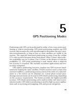
INTRODUCTION(1-13)

This book presents detailed information in a compact form about the global
positioning system (GPS) coarse/acquisition (C/ A) 'code receiver. Using the
C/ A code to find the user location is referred to as the standard position service
(SPS). Most of the information can be found in references 1 through 13. However, there is much more information in the references than the basics required
to understand a GPS receiver. Therefore, one must study the proper subjects
and put them together. This is a tedious and cumbersome task. This book does
this job for the reader.
This book not only introduces the information available from the references,
it emphasizes its applications. Software programs are provided to help understand some of the concepts. These programs are also useful in designing GPS
receivers. In addition, various techniques to perform acquisition and tracking
on the GPS signals are included.
This book concentrates only on the very basic concepts of the C/ A code
GPS receiver. Any subject not directly related to the basic receiver (even if
it is of general interest, i.e., differential GPS receiver and GPS receiver with
carrier-aided tracking capacity) will not be included in this book. These other
subjects can be found in reference I.

1.2

HISTORY OF GPS DEVELOPMENT(1,5,12)

The discovery of navigation seems to have occurred early in human history.
According to Chinese storytelling, the compass was discovered and used in wars
during foggy weather before recorded history. There have been many different
navigation techniques to support ocean and air transportation. Satellite-based
navigation started in the early 1970s. Three satellite systems were explored
1


2

before the GPS programs: the U.S. Navy Navigation Satellite System (also
referred to as the Transit), the U.S. Navy's Timation (TIMe navigATION), and
U.S. Air Force project 621B. The Transit project used a continuous wave (cw)
signal. The closest approach of the satellite can be found by measuring the
maximum rate of Doppler shift. The Timation program used an atomic clock
that improves the prediction of satellite orbits and reduces the ground control
update rate. The Air Force 621B project used the pseudorandom noise (PRN)
signal to modulate the carrier frequency.
The GPS program was approved in December 1973. The first satellite was
launched in 1978. In August 1993, GPS had 24 satellites in orbit and in December of the same year the initial operational capability was established. In February
1994, the Federal Aviation Agency (FAA) declared GPS ready for aviation use.

1.3

1.4

INTRODUCTION

A BASIC GPS RECEIVER

The basic GPS receiver discussed in this book is shown in Figure 1.1. The signals transmitted from the GPS satellites are received from the antenna. Through
the radio frequency (RF) chain the input signal is amplified to a proper amplitude and the frequency is converted to a desired output frequency. An analogto-digital converter (ADC) is used to digitize the output signal. The antenna,
RF chain, and ADC are the hardware used in the receiver.
After the signal is digitized, software is used to process it, and that is why this
book has taken a software approach. Acquisition means to find the signal of a
certain satellite. The tracking program is used to find the phase transition of the
navigation data. In a conventional receiver, the acquisition and tracking are performed by hardware. From the navigation data phase transition the subframes
and navigation data can be obtained. Ephemeris data and pseudoranges can be

APPROACHES OF PRESENTATION

3

obtained from the navigation data. The ephemeris data are used to obtain the
satellite positions. Finally, the user position can be calculated for the satellite
positions and the pseudoranges. Both the hardware used to collect digitized data
and the software used to find the user position will be discussed in this book.

1.4

APPROACHES OF PRESENTATION

There are two possible approaches to writing this book. One is a straightforward
way to follow the signal flow shown in Figure 1.1. In this approach the book
would start with the signal structure of the GPS system and the methods to process the signal to obtain the necessary the information. This information would
be used to calculate the positions of the satellites and the pseudoranges. By
using the positions of the satellites and the pseudoranges the user position can
be found. In this approach, the flow of discussion would be smooth, from one
subject to another. However, the disadvantage of this approach is that readers
might not have a clear idea why these steps are needed. They could understand

the concept of the GPS operation only after reading the entire book.
The other approach is to start with the basic 'concept of the GPS from a
system designers' point of view. This approach wou1d start with the basic concept of finding the user position from the satellite positions. The description
of the satellite constellation would be presented. The detailed information of
the satellite orbit is contained in the GPS data. In order to obtain these data,
the GPS signal must be tracked. The C/ A code of the GPS signals would then
be presented. Each satellite has an unique C/ A code. A receiver can perform
acquisition on the C/ A code to find the signal. Once the C/ A code of a certain
satellite is found, the signal can be tracked. The tracking program can produce
the navigation data. From these data, the position of the satellite can be found.
The relative pseudorange can be obtained by comparing the time a certain data
point arrived at the receiver. The user position can be calculated from the satellite positions and pseudoranges of several satellites.
This book takes this second approach to present the material because it
should give a clearer idea of the GPS function from the very beginning. The
final chapter describes the overall functions of the GPS receiver and can be
considered as taking the first approach for digitizing the signal, performing
acquisition and tracking, extracting the navigation data, and calculating the user
position.

1.5

SOFTWARE APPROACH

This book uses the concept of software radio to present the subject. The software radio idea is to use an analog-to-digital converter (ADC) to change the
input signal into digital data at the earliest possible stage in the receiver. In
other words, the input signal is digitized as close to the antenna as possible.


4

1.7

INTRODUCTION

Once the signal is digitized, digital signal processing will be used to obtain
the necessary information. The primary goal of the software radio is minimum
hardware use in a radio. Conceptually, one can tune the radio through software
or even change the function of the radio such as from amplitude modulation
(AM) to frequency modulation (FM) by changing the software; therefore great
flexibility can be achieved.
The main purpose of using the software radio concept to present this subject
is to illustrate the idea of signal acquisition and tracking. Although using hardware to perform signal acquisition and tracking can also describe GPS receiver
function, it appears that using software may provide a clearer idea of the signal acquisition and tracking. In addition, a software approach should provide a
better understanding of the receiver function because some of the calculations
can be illustrated with programs. Once the software concept is well understood,
the readers should be able to introduce new solutions to problems such as various acquisition and tracking methods to improve efficiency and performance.
At the time (December 1997) this chapter was being written, a software GPS
receiver using a 200 MHz personal computer (PC) could not track one satellite
in real time. When this chapter was revised in December 1998, the software
had been modified to track two satellites in real time with a new PC operating at 400 MHz. Although it is still impossible to implement a software GPS
receiver operating in real time, with the improvement in PC operating speed and
software modification it is likely that by the time this book is published a software GPS receiver will be a reality. Of course, using a digital signal processing
(DSP) chip is another viable way to build the receiver.
Only the fundamentals of a GPS receiver are presented in this book. In order
to improve the performance of a receiver, fine tuning of some of the operations
might be necessary. Once readers understand the basic operation principles of
the receiver, they can make the necessary improvement.

1.6

POTENTIAL ADVANTAGES

OF THE SOFTWARE

APPROACH

An important aspect of using the software approach to build a GPS receiver
is that the approach can drastically deviate from the conventional hardware
approach. For example, the user may take a snapshot of data and process' them
to find the location rather than continuously tracking the signal. Theoretically,
30 seconds of data are enough to find the user location. This is especially useful when data cannot be collected in a continuous manner. Since the software
approach is in the infant stage, one can explore many potential methods.
The software approach is very flexible. It can process data collected from
various types of hardware. For example, one system may collect complex data
referred to as the inphase and quadrature-phase (I and Q) channels. Another
system may collect real data from one channel. The data can easily be changed
from one form to another. One can also generate programs to process complex
signals from programs processing real signals or vice versa with some simple

ORGANIZATION OF THE BOOK

5

modifications. A program can be used to process signals digitized with various
sampling frequencies. Therefore, a software approach can almost be considered
as hardware independent.
New algorithms can easily be developed without changing the design of the
hardware. This is especially useful for studying some new problems. For example, in order to study the antijamming problem one can collect a set of digitized
signals with jamming signals present and use different algorithms to analyze it.

1.7

ORGANIZATION

OF THE BOOK

This book contains nine chapters. Chapter 2 introduces the user position requirements, which lead to the GPS parameters. Also included in Chapter 2 is the basic
concept of how to find the user position if the satellite positions are known. Chapter 3 discusses the satellite constellation and its impact on the GPS signals, which
in turn affects the design of the GPS receiver. Chapter 4 discusses the earth-centered, earth-fixed system. Using this coordinate system, the user position can be
calculated to match the position on every-day maps. The GPS signal structure is
discussed in detail in Chapter 5. Chapter 6 discusses th~ hardware to collect data,
which is equivalent to the front end of a conventional GPS receiver. Changing the
format of data is also presented. Chapter 7 presents several acquisition methods.
Some of them can be used in hardware design and others are suitable for software applications. Chapter 8 discusses two tracking methods. One uses the conventional phase-locked loop approach and the other one is more suitable for the
software radio approach. The final chapter is a summary ofthe previous chapters.
It takes all the information in the first eight chapters and presents in it an order
following the signal flow in a GPS receiver ..
Computer programs written in Matlab are listed at the end of several chapters. Some of the programs are used only to illustrate ideas. Others can be used
in the receiver design. In the final chapter all of the programs related to designing a receiver will listed. These programs are by no means optimized and they
are used only for demonstration purposes.

REFERENCES
1. Parkinson, B. W., Spilker, J. J. Jr., Global Positioning System: Theory and Applications, vols. I and 2, American Institute of Aeronautics and Astronautics, 370
L'Enfant Promenade, SW, Washington, DC, 1996.
2. "System specification for the navstar global positioning system," SS-GPS-300B
code ident 07868, March 3, 1980.
3. Spilker, J. J., "GPS signal structure and performance characteristics," Navigation,
Institute of Navigation, vol. 25, no. 2, pp. 121-146, Summer 1978.
4. Milliken, R. J., Zoller, C. J., "Principle of operation of NAVSTAR and system characteristics," Advisory Group for Aerospace Research and Development (AGARD)

6

INTRODUCTION

Ag-245, pp. 4-1-4.12, July 1979.
5. Misra, P. N., "Integrated use of GPS and GLONASS in civil aviation," Lincoln Laboratory Journal, Massachusetts Institute of Technology, vol. 6, no. 2, pp. 231-247,
Summer/Fall, 1993.
6. "Reference data for radio engineers," 5th ed., Howard W. Sams & Co. (subsidiary
of ITT), Indianapolis, 1972.
7. Bate, R. R., Mueller, D. D., White, J. E., Fundamentals of Astrodynamics, pp.
182-188, Dover Publications, New York, 1971.
8. Wells, D. E., Beck, N., Delikaraoglou, D., Kleusbery, A., Krakiwsky, E. J.,
Lachapelle, G., Langley, R. B., Nakiboglu, M., Schwarz, K. P., Tranquilla, J. M.,
Vanicek, P., Guide to GPS Positioning, Canadian GPS Associates, Frederiction,
N.H., Canada, 1987.
9. "Department of Defense world geodetic system, 1984 (WGS-84), its definition and
relationships with local geodetic systems," DMA-TR-8350.2, Defense Mapping
Agency, September 1987.
10. "Global Positioning System Standard Positioning Service Signal Specification, 2nd
ed., GPS Joint Program Office, June 1995.
II. Bate, R. R., Mueller, D. D., White, J. E., Fundamentals of Astrodynamics, Dover
Publications, New York, 1971.
12. Riggins, B., "Satellite navigation using the global positioning system," manuscript
used in Air Force Institute of Technology, Dayton OH, 1996.
13. Kaplan, E. D., ed., Understanding GPS Principles and Applications, Artech House,
Norwood, MA, 1996.

Basic GPS Concept

2.1

INTRODUCTION

This chapter will introduce the basic concept of how 1\ GPS receiver determines
its position. In order to better understand the concept, GRS performance requirements will be discussed first. These requirements determine the arrangement of
the satellite constellation. From the satellite constellation, the user position can
be solved. However, the equations required for solving the user position turn
out to be nonlinear simultaneous equations, which are difficult to solve directly.
In addition, some practical considerations (i.e., the inaccuracy of the user clock)
will be included in these equations. These equations are solved through a linearization and iteration method. The solution is in a Cartesian coordinate system
and the result will be converted into a spherical coordinate system. However,
the earth is not a perfect sphere; therefore, once the user position is found, the
shape of the earth must be taken into consideration. The user position is then
translated into the earth-based coordinate system. Finally, the selection of satellites to obtain better user position accuracy and the dilution of precision will
be discussed.

2.2

GPS PERFORMANCE

REQUIREMENTS(1)

Some of the performance requirements are listed below:
1. The user position root mean square (rms) error should be 10-30 m.
2. It should be applicable to real-time navigation for all users including the
high-dynamics user, such as in high-speed aircraft with flexible maneuverability.
3. It should have worldwide coverage. Thus, in order to cover the polar
regions the satellites must be in inclined orbits.
7

8

BASIC GPS CONCEPT

4. The transmitted signals should tolerate, to some degree, intentional
and unintentional interference. For example, the harmonics from some
narrow-band signals should not disturb its operation. Intentional jamming
of GPS signals is a serious concern for military applications.
5. It cannot require that every GPS receiver utilize a highly accurate clock
such as those based on atomic standards.
6. When the receiver is first turned on, it should take minutes rather than
hours to find the user position.
7. The size of the receiving antenna should be small. The signal attenuation
through space should be kept reasonably small.
These requirements combining with the availability of the frequency band
allocation determines the carrier frequency of the GPS to be in the L band (1-2
GHz) of the microwave range.

2.3

BASIC GPS CONCEPT

The position of a certain point in space can be found from distances measured
from this point to some known positions in space. Let us use some examples to
illustrate this point. In Figure 2.1, the user position is on the x-axis; this is a onedimensional case. If the satellite position S I and the distance to the satellite x I
are both known, the user position can be at two places, either to the left or right
of S,. In order to determine the user position, the distance to another satellite
with known position must be measured. In this figure, the positions of S2 and

X2 uniquely determine the user position U.
Figure 2.2 shows a two-dimensional case. In order to determine the user
position, three satellites and three distances are required. The trace of a point
with constant distance to a fixed point is a circle in the two-dimensional case.
Two satellites and two distances give two possible solutions because two circles
intersect at two points. A third circle is needed to uniquely determine the user
position.
For similar reasons one might decide that in a three-dimensional case four
satellites and four distances are needed. The equal-distance trace to a fixed point
is a sphere in a three-dimensional case. Two spheres intersect to make a circle.
This circle intersects another sphere to produce two points. In order to determine
which point is the user position, one more satellite is needed.

In GPS the position of the satellite is known from the ephemeris data transmitted by the satellite. One can measure the distance from the receiver to the
satellite. Therefore, the position of the receiver can be determined.
In the above discussion, the distance measured from the user to the satellite
is assumed to be very accurate and there is no bias error. However, the distance
measured between the receiver and the satellite has a constant unknown bias,
because the user clock usually is different from the GPS clock. In order to
resolve this bias error one more satellite is required. Therefore, in order to find
the user position five satellites are needed.
If one uses four satellites and the measured distance with bias error to measure a user position, two possible solutions can be obtained. Theoretically, one
cannot determine the user position. However, one of the solutions is close to the
earth's surface and the other one is in space. Since the user position is usually
close to the surface of the earth, it can be uniquely determined. Therefore, the
general statement is that four satellites can be used to determine a user position,
even though the distance measured has a bias error.
The method of solving the user position discussed in Sections 2.5 and 2.6
is through iteration. The initial position is often selected at the center of the
earth. The iteration method will converge on the correct solution rather than

10

BASIC GPS CONCEPT

the one in space. In the following discussion four satellites are considered the
minimum number required in finding the user position.

2.4

BASIC EQUATIONS

FOR FINDING

USER POSITION

In this section the basic equations for determining the user position will be presented. Assume that the distance measured is accurate and under this condition
three satellites are sufficient. In Figure 2.3, there are three known points at locations r] or (Xl, Yl, zd, r2 or (X2, Y2, Z2), and r3 or (X3, Y3, Z3), and an unknown
point at r u or (xu, Yu, zu). If the distances between the three known points to
the unknown point can be measured as PI, P2, and P3, these distances can be
written as

Because there are three unknowns and three equations, the values of Xu, Yu,
and Zu can be determined from these equations. Theoretically, there should be




2.9

EARTH GEOMETRy(4-6)

The earth is not a perfect sphere but is an ellipsoid; thus, lhe latitude and altitude
calculated from Equations (2.18) and (2.20) must be modified. However, the
longitude I calculated from Equation (2.19) also applies to the nonspherical
earth. Therefore, this quantity does not need modification. Approximations will
be used in the following discussion, which is based on references 4 through 6.
For an ellipsoid, there are two latitudes. One is referred to as the geocentric
latitude L" which is calculated from the previous section. The other one is the
geodetic latitude L and is the one often used in every-day maps. Therefore, the
geocentric latitude must be converted to the geodetic latitude. Figure 2.5 shows
a cross section of the earth. In this figure the x-axis is along the equator, the
'y-axis is pointing inward to the paper, and the z-axis is along the north pole of
the earth. Assume that the user position is on the x-z plane and this assumption
does not lose generality. The geocentric latitude Lc is obtained by drawing a
line from the user to the center of the earth, which is calculated from Equation
(2.18).
The geodetic latitude is obtained by drawing a line perpendicular to the surface of the earth that does not pass the center of the earth. The angle between
'this line and the x is the geodetic latitude L. The height of the user is the distance h perpendicular and above the surface of the earth.
The following discussion is used to determine three unknown quantities from
two known quantities. As shown in Figure 2.5, the two known quantities are
the distance r and the geocentric latitude Lc and they are measured from the
ideal spherical earth. The three unknown quantities are the geodetic latitude
L, the distance ra, and the height h. All three quantities are calculated from
approximation methods. Before the actual calculations of the unknowns, let us
introduce some basic relationships in an ellipse.

2.14

SATELLITE SELECTION(1,8)

A GPS receiver can simultaneously receive signals from 4 up to 11 satellites,
if the receiver is on the surface of the earth. Under this condition, there are
two approaches to solve the problem. The first one is to use all the satellites to
calculate the user position. The other approach is to choose only four satellites
from the constellation. The usual way is to utilize all the satellites to calculate
the user position, because additional measurements are used. In this section and
section 2.15 the selection of satellites will be presented. In order to focus on
this subject only the four-satellite case will be considered.
If there are more than four satellite signals that can be received by a GPS
receiver, a simple way is to choose only four satellites and utilize them to solve
for the user position. Under this condition, the question is how to select the four
satellites. Let us use a two-dimensional case to illustrate the situation, because
it is easier to show graphically. In order to solve a position in a two-dimensional case, three satellites are required considering the user clock bias. In this
discussion, it is assumed that the user position can be uniquely determined as
discussed in Section 2.3. If this assumption cannot be used, four satellites are
required.
Figure 2.8a shows the results measured by three satellites on a straight line,
and the user is also on this line. Figure 2.8b shows that the three satellites


2.15

DILUTION OF I'~ECISI()N

27

and the user form a quadrangle. Two circles with the same center but different
radii am drawn. The solid circle represents the distance measured from the user
to the satellite with bias clock error. The dotted circle represents the distance
after the clock error correction. From observation, the position error in Figure
'2.8a is greater than that in Figure 2.8b. because in Figure 2.8a all three dotted
circles are tangential to each other. It is difficult to measure the tangential point
accurately. In Figure 2.8b, the three circles intersect each other and the point
of intersection can be measured more accurately. Another way to view this
problem is to measure the area of a triangle made by the three satellites. In
Figure 2.8a the total area is close to z~o, while in Figure 2.8b the total area is
quite large. In general, the larger the triangle area made by the three satellites,
the better the user position can be solved.
The general rule can be extended to select the four satellites in a three-dimensional case. It is desirable to maximize the volume defined by the four satellites.
A tetrahedron with an equilateral base contains the maximum volume and therefore can be considered as the best selection. Under this condition, one satellite
is at zenith and the other three are close to the horizon and separated by 120
degrees.(8) This geometry will generate the best user position estimation. If all
four satellites are close to the horizon, the volume defined by these satellites
and the user is very small. Occasionally, the user positidn error calculated with
this arrangement can be extremely large. In other words, the DU calculated from
Equation (2.11) may not converge.

2.15

DILUTION OF PRECISION(1,8)

The dilution of precision (OOP) is often used to measure user position accuracy.
There are several different definitions of the OOP. All the different OOPs are
a function of satellite geometry only. The positions of the satellites determine

the OOP value. A detailed discussion can be found in reference 8. Here only
the definitions and the limits of the values will be presented.
The geometrical dilution of precision (GOOP) is defined as


2. Spilker, J. J. Jr., Parkinson, B. w., "Overview of GPS operation and design," Chapter 2, and Spilker, J. J. Jr., "GPS navigation data," Chapter 4 in Parkinson, B. w.,
Spilker, J. J. Jr., Global Positionin~ System: Theory and Applications, vols. I and
2, American Institute of Aeronautics and Astronautics, 370 L'Enfant Promenade,
SW, Washington, DC, 1996.
3. Kay, S. M., Fundamentals of Stati.l'timl Sixnal Pro('e.l'.I'in~ Estimation Theory, Chapter 8, Prentice HaIl, Englewood Cliffs, NJ 1993.
4. Bate, R. R., MuelIer, D. D., and White, 1. E., Fundamentals of Astrodynamics,
Chapter 5, Dover Publications, New York, 1971.
5. Britting, K. R., Inertial Navigation Sy.\'tems Analysis, Chapter 4, Wiley, 1971.
6. Riggins, R. "Navigation using the global positioning system," Chapter 6, class
notes, Air Force Institute of Technology, 1996.
7. "Department of Defense world geodetic system, 1984 (WGS-84), its definition and
relationships with local geodetic systems," DMA-TR-8350.2, Defense Mapping
Agency, September 1987.
8. Spilker, J. J. Jr., "SateIlite constellation and geometric dilution of precision," Chapter 5, and Axelraq, P., Brown, R. G., "GPS navigation algorithms," Chapter 9 in
Parkinson, B. W., Spilker, 1. J. Jr., Global Positioning System: Theory and Applications, vols. I and 2, American Institute of Aeronautics and Astronautics, 370
L'Enfant Promenade, SW, Washington, DC, 1996.


30

REFERENCES

BASIC GPS CONCEPT

%p2_1.m

%Userpos. muse pseudorange
position
%JT 30 April 96
% *****

Input data *****

sp(1:3,

l:nsat);

%satellite

and satellite

position

positions

to calcuiate

which has the following

user

format

end
drao = pr - (rao + ones(l,nsat)*bu)

;%** find delta rao
% includes clock bias
(2.16)

dl = pinv(h)*drao';
%Equation
bu = bu + dl (4); %new clock bias
for k = 1: 3;
gu (k) = gu (k) + dl (k) ; %**find new posi tion
end
erro=dl(1)1\2+dl(2)1\2+dl(3)1\2;
%find error
for j = l:nsat;
rao(j)=((gu(1)-sp(1,j))1\2+(gu(2)-sp(2,j))1\2+(gu(3)sp (3, j) )1\2) 1\.5; %find new rao without
end
end
%***** Final

result

in spherical

coordinate

clock bias

system *****

xuser = gu (1) ; yuser = gu (2) ; zuser = gu (3) ; bias = bu;

.

pr(l:nsat);
%is the measured pseudo-range
% pr= [pr1 pr2 pr3 ...
prnn] T;
nn=nsat;

which has the format as

% is the number of satellites

% ***** Select initial
guessed positions
and clock
x_guess = 0; y_guess = 0; z_guess = 0; bu = 0;

gU(l) = x_guess;

gu(2) = y_guess;

% Calculating
rao the pseudo-range
%clock bias is not included
for j = l:nsat
rao(j)=((gu(1)-sp(1,j))1\2+(gu(2)-sp(2,j)
- sp (3 , j ) ) 1\ 2 ) 1\ . 5 ;
end

bias

*****

gu(3) = z_guess;

rsp = (xuser"2+yuserI\2+zuserI\2)1\.5;

%radius otspherical
earth
%Eq 2 . 17
Lc = atan(zuser/(xuserI\2+yuserI\2)1\.5);
% latitude
of spherical
% earth Eq 2.18
lsp = atan(yuser/xuser)
*180/pi; % longitude
spherical
and flat
% earth Eq 2. 19
% ***** Converting

as shown in Equation

(2.1)

the

to practical

earth

shape *****

e=1/298.257223563;
Ltemp=Lc;
erro1=1;

)1\2+(gu(3)

% generate
the fourth column of the alpha matrix
alpha ( : ,4) = ones(nsat,l);

in Eq. 2.15

erro=l i
while erro2.. 01; .
for j = 1 :nsat;
for k = 1: 3;
alpha (j ,k) = (gu (k) -sp (k, j)) / (rao (j)) ; % find first
%3 columns of alpha matrix
end

while erro1>le-6;
% calculating
latitude
by Eq. 2.51
L=Lc+e*sin(2*Ltemp) ;
erro1=abs(Ltemp-L)
;

Ltemp=L;
end
Lflp=L*180/pi; % latitude
of flat earth
re=6378137 ;
h=rsp-re*
(l-e* (sin(L) 1\2));
%altitude
of flat earth
lsp = lsp; % longitude
of flat earth
upos = [xuser yuser zuser bias rsp Lflp lsp h] , ;

31


3.2

3.2

Satellite Constellation

3.1

INTRODUCTION

The previous chapter assumes that the positions of the satellites are known.
This chapter will discuss the satellite constellation and the determination of the
satellite positions. Some special terms related to the orbital mechanics, such as
sidereal day, will be introduced. The satellite motion will have an impact on

the processing of the signals at the receiver. For example, the input frequency
shifts as a result of the Doppler effect. Such details are important for the design
of acquisition and tracking loops in the receiver. However, in order to obtain
some of this information a very accurate calculation of the satellite motion is not
needed. For example, the actual orbit of the satellite is elliptical but it is close
to a circle. The information obtained from a circular orbit will be good enough
to find an estimation of the Doppler frequency. Based on this assumption the
circular orbit is used to calculate the Doppler frequency, the rate of change of
the Doppler frequency, and the differential power level. From the geometry of
the satellite distribution, the power level at the receiver can also be estimated
from the transmission power. This subject is presented in the final section in this
chapter .•
In order to find the location of the satellite accurately, a circular orbit is insufficient. The actual elliptical satellite orbit must be used. Therefore, the complete
elliptical satellite orbit and Kepler's law will be disGussed. Information obtained
from the satellite through the GPS receiver via broadcast navigation data such
as the mean anomaly does not provide the location of the satellite directly.
However, this infofmation can be used to calculate the precision location of
the satellite. The calculation of the satellite position from these data will be
discussed in detail.

32

CONTROL

SEGMENT

CONTROL

SEGMENT

OF THE GPS SYSTEM

33

OF THE GPS SYSTEM(1-3)

This section will provide a very brief idea of the GPS system. The GPS system may be considered as comprising three segments: the control segment, the
space segment, and the user segment. The space segment contains all the satellites, which will be discussed in Chapters 3, 4, and 5. The user segment' can
be considered the base of receivers and their processing, which is the focus of
this text. The control segment will be discussed in this section.
The control segment consists of five control stations, including a master control station. These control stations are widely separated in longitude around the
earth. The master control station is located at Falcon Air Force Base, Colorado
Springs, CO. Operations are maintained at all times year round. The main purpose of the control stations is to monitor the performance of the GPS satellites.
The data collected from the satellites by the control stations will be sent to
the master control station for processing. The master control station is responsible for all aspects of constellation control and command. A few of the operation objectives are presented here: (1) Monitor GPS performance in support
of all performance standards. (2) Generate and upload the navigation data to
the satellites to sustain performance standards. (3) Pr?mptly detect and respond
to satellite failure to minimize the impact. Detailed inftJrmation on the control
segment can be found in reference 3.

3.3

SATELLITE CONSTELLATlON(3-9)

There are a total of24 GPS satellites divided into six orbits and each orbit has four
satellites. Each orbit makes a 55-degree angle with the equator, which is referred
to as the inclination angle. The orbits are separated by 60 degrees to cover the
complete 360 degrees. The radius of the satellite orbit is 26,560 km and it rotates
around the earth twice in a sidereal day. Table 3.1 lists all these parameters.
The central body of the Block IIR satellite is a cube of approximately 6 ~t

on each side.(8) The span of the solar panel is about 30 ft. The lift-off weight
of the spacecraft is 4,480 pounds and the on-orbit weight is 2,370 pounds.

TABLE 3.1

Characteristics of GPS Satellites
Constellation

Number of satellites
Number of orbital planes
Number of satellites per orbit
Orbital inclination
Orbital radius(7)
Period(4)
Ground track repeat

24
6
4
55°
26560 km
II hrs 57 min 57.26 see

sidereal day