Financial modeling a backward stochastic differential equations perspective, crepey
Bạn đang xem bản rút gọn của tài liệu. Xem và tải ngay bản đầy đủ của tài liệu tại đây (4.65 MB, 463 trang )
Springer Finance
Textbooks
Stéphane Crépey
Financial
Modeling
A Backward Stochastic
Differential Equations Perspective
Springer Finance
Textbooks
Editorial Board
Marco Avellaneda
Giovanni Barone-Adesi
Mark Broadie
Mark H.A. Davis
Emanuel Derman
Claudia Klüppelberg
Walter Schachermayer
Springer Finance Textbooks
Springer Finance is a programme of books addressing students, academics and
practitioners working on increasingly technical approaches to the analysis of financial markets. It aims to cover a variety of topics, not only mathematical finance but
foreign exchanges, term structure, risk management, portfolio theory, equity derivatives, and financial economics.
This subseries of Springer Finance consists of graduate textbooks.
For further volumes:
/>
Stéphane Crépey
Financial
Modeling
A Backward Stochastic
Differential Equations Perspective
Prof. Stéphane Crépey
Département de mathématiques,
Laboratoire Analyse & Probabilités
Université d’Evry Val d’Essone
Evry, France
Additional material to this book can be downloaded from
Password: [978-3-642-37112-7]
ISBN 978-3-642-37112-7
ISBN 978-3-642-37113-4 (eBook)
DOI 10.1007/978-3-642-37113-4
Springer Heidelberg New York Dordrecht London
Library of Congress Control Number: 2013939614
Mathematics Subject Classification: 91G20, 91G60, 91G80
JEL Classification: G13, C63
© Springer-Verlag Berlin Heidelberg 2013
This work is subject to copyright. All rights are reserved by the Publisher, whether the whole or part of
the material is concerned, specifically the rights of translation, reprinting, reuse of illustrations, recitation,
broadcasting, reproduction on microfilms or in any other physical way, and transmission or information
storage and retrieval, electronic adaptation, computer software, or by similar or dissimilar methodology
now known or hereafter developed. Exempted from this legal reservation are brief excerpts in connection
with reviews or scholarly analysis or material supplied specifically for the purpose of being entered
and executed on a computer system, for exclusive use by the purchaser of the work. Duplication of
this publication or parts thereof is permitted only under the provisions of the Copyright Law of the
Publisher’s location, in its current version, and permission for use must always be obtained from Springer.
Permissions for use may be obtained through RightsLink at the Copyright Clearance Center. Violations
are liable to prosecution under the respective Copyright Law.
The use of general descriptive names, registered names, trademarks, service marks, etc. in this publication
does not imply, even in the absence of a specific statement, that such names are exempt from the relevant
protective laws and regulations and therefore free for general use.
While the advice and information in this book are believed to be true and accurate at the date of publication, neither the authors nor the editors nor the publisher can accept any legal responsibility for any
errors or omissions that may be made. The publisher makes no warranty, express or implied, with respect
to the material contained herein.
Printed on acid-free paper
Springer is part of Springer Science+Business Media (www.springer.com)
To Irène and Camille
Preface
This is a book on financial modeling that emphasizes computational aspects. It gives
a unified perspective on derivative pricing and hedging across asset classes and is
addressed to all those who are interested in applications of mathematics to finance:
students, quants and academics.
The book features backward stochastic differential equations (BSDEs), which
are an attractive alternative to the more familiar partial differential equations (PDEs)
for representing prices and Greeks of financial derivatives. First, BSDEs offer the
most unified setup for presenting the financial derivatives pricing and hedging theory
(as reflected by the relative compactness of the book, given its rather wide scope).
Second, BSDEs are a technically very flexible and powerful mathematical tool for
elaborating the theory with all the required mathematical rigor and proofs. Third,
BSDEs are also useful for the numerical solution of high-dimensional nonlinear
pricing problems such as the nonlinear CVA and funding issues which have become
important since the great crisis [30, 80, 81].
Structure of the Book
Part I provides a course in stochastic processes, beginning at a quite elementary
level in order to gently introduce the reader to the mathematical tools that are needed
subsequently. Part II deals with the derivation of the pricing equations of financial
claims and their explicit solutions in a few cases where these are easily obtained, although typically these equations have to be solved numerically as is done in Part III.
Part IV provides two comprehensive applications of the book’s approach that illustrate the versatility of simulation/regression pricing schemes for high-dimensional
pricing problems. Part V provides a thorough mathematical treatment of the BSDEs
and PDEs that are of fundamental importance for our approach. Finally, Part VI is
an extended appendix with technical proofs, exercises and corrected problem sets.
vii
viii
Preface
Outline
Chapters 1–3 provide a survey of useful material from stochastic analysis. In Chap. 4
we recall the basics of financial theory which are necessary for understanding how
the risk-neutral pricing equation of a generic contingent claim is derived. This chapter gives a unified view on the theory of pricing and hedging financial derivatives,
using BSDEs as a main tool. We then review, in Chap. 5, benchmark models on
reference derivative markets. Chapter 6 is about Monte Carlo pricing methods and
Chaps. 7 and 8 deal with deterministic pricing schemes: trees in Chap. 7 and finite
differences in Chap. 8.
Note that there is no hermetic frontier between deterministic and stochastic pricing schemes. In essence, all these numerical schemes are based on the idea of propagating the solution, starting from a surface of the time-space domain on which it
is known (typically: the maturity of a claim), along suitable (random) “characteristics” of the problem. Here “characteristics” refers to Riemann’s method for solving
hyperbolic first-order equations (see Chap. 4 of [191]). From the point of view of
control theory, all these numerical schemes can be viewed as variants of Bellman’s
dynamic programming principle [26]. Monte Carlo pricing schemes may thus be regarded as one-time-step multinomial trees, converging to a limiting jump diffusion
when the number of space discretization points (tree branches) goes to infinity. The
difference between a tree method in the usual sense and a Monte Carlo method is
that a Monte Carlo computation mesh is stochastically generated and nonrecombining.
Prices of liquid financial instruments are given by the market and are determined
by supply-and-demand. Liquid market prices are thus actually used by models in the
“reverse-engineering” mode that consists in calibrating a model to market prices.
This calibration process is the topic of Chap. 9. Once calibrated to the market, a
model can be used for Greeking and/or for pricing more exotic claims (Greeking
means computing risk sensitivities in order to set-up a related hedge).
Analogies and differences between simulation and deterministic pricing schemes
are most clearly visible in the context of pricing by simulation claims with early exercise features (American and/or cancelable claims). Early exercisable claims can
be priced by hybrid “nonlinear Monte Carlo” pricing schemes in which dynamic
programming equations, similar to those used in deterministic schemes, are implemented on stochastically generated meshes. Such hybrid schemes are the topics of
Chaps. 10 and 11, in diffusion and in pure jump setups, respectively. Again, this is
presently becoming quite topical for the purpose of CVA computations.
Chapters 12–14 develop, within a rigorous mathematical framework, the connection between backward stochastic differential equations and partial differential
equations. This is done in a jump-diffusion setting with regime switching, which
covers all the models considered in the book.
Finally Chap. 15 gathers the most demanding proofs of Part V, Chap. 16 is devoted to exercises for Part I and Chap. 17 provides solved problem sets for Parts II
and III.
Preface
ix
Fig. 1 Getting started with the book: roadmap of “a first and partial reading” for different audiences. Green: Students. Blue: Quants. Red: Academics
Roadmap
Given the dual nature of the proposed audience (scholars and quants), we have provided more background material on stochastic processes, pricing equations and numerical methods than is needed for our main purposes. Yet we have not avoided the
sometimes difficult mathematical technique that is needed for deep understanding.
So, for the convenience of readers, we signal sections that contain advanced material with an asterisk (*) or even a double asterisk (**) for the still more difficult
portions.
Our ambition is, of course, that any reader should ultimately benefit from all
parts of the book. We expect that an average reader will need two or three attempts
at reading at different levels for achieving this objective. To provide additional guidance, we propose the following roadmap of what a “first and partial” reading of the
book could be for three “stylized” readers (see Fig. 1 for a pictorial representation):
a student (in “green” on the figure), a quant (“blue” audience) and an academic
(“red”; the “blue and red” box in the chart may represent a valuable first reading for
both quants and academics):
• for a graduate student (“green”), we recommend a first reading of the book at
a classical quantitative and numerical finance textbook level, as follows in this
order:
– start by Chaps. 1–3 (except for the starred sections of Chap. 3), along with the
accompanying (generally classical) exercises of Chap. 16,1
1 Solutions
of the exercises are available for course instructors.
x
Preface
– then jump to Chaps. 5 to 9, do the corrected problems of Chap. 17 and run the
accompanying Matlab scripts ();
• for a quant (“blue”):
– start with the starred sections of Chap. 3, followed by Chap. 4,
– then jump to Chaps. 10 and 11;
• for an academics or a PhD student (“red”):
– start with the starred sections of Chap. 3, followed by Chap. 4,
– then jump to Chaps. 12 to 14, along with the related proofs in Chap. 15.
The Role of BSDEs
Although this book isn’t exclusively dedicated to BSDEs, it features them in various
contexts as a common thread for guiding readers through theoretical and computational aspects of financial modeling. For readers who are especially interested in
BSDEs, we recommend:
•
•
•
•
Section 3.5 for a mathematical introduction of BSDEs at a heuristic level,
Chapter 4 for their general connection with hedging,
Section 6.10 and Chap. 10 for numerical aspects and
Part V and Chap. 15 for the related mathematics.
In Sect. 11.5 we also give a primer of CVA computations using simulation/regression
techniques that are motivated by BSDE numerical schemes, even though no BSDEs
appear explicitly. More on this will be found in [30], for which the present book
should be a useful companion.
Bibliographic Guidelines
To conclude this preface, here are a few general references:
• on random processes and stochastic analysis, often with connections to finance
(Chaps. 1–3): [149, 159, 167, 174, 180, 205, 228];
• on martingale modeling in finance (Chap. 4): [93, 114, 159, 191, 208, 245];
• on market models (Chap. 5): [43, 44, 58, 131, 146, 208, 230, 241];
• on Monte Carlo methods (Chap. 6): [133, 176, 226];
• on deterministic pricing schemes (Chaps. 7 and 8): [1, 12, 27, 104, 172, 174, 207,
248, 254, 256];
• on model calibration (Chap. 9): [71, 116, 213];
• on simulation/regression pricing schemes (Chaps. 10 and 11): [133, 136];
• on BSDEs and PDEs, especially in connection with finance (Chaps. 12–14): [96,
113, 114, 122, 164, 197, 224].
Preface
xi
Acknowledgements2
This book grew out of various courses that I taught for many years in different
quantitative finance master programs, starting with the one of my home university
of Evry (MSc “M2IF”). I would like to thank all the students, who provided useful
feedback through their questions and comments. The book also has a clear flavor
of long run collaboration with my colleagues and friends Monique Jeanblanc, Tom
Bielecki and Marek Rutkowski. A course given by Tom Bielecki at Illinois Institute
of Technology was used as the basis of a first draft for Part I. Chapters 6–8 rely to
some extent on the documentation of the option pricing software PREMIA developed since 1999 at INRIA and CERMICS under the direction of Bernard Lapeyre,
Agnès Sulem and Antonino Zanette (see www.premia.fr); I thank Claude Martini
and Katia Voltchkova for having let me use their contributions to PREMIA in preliminary versions of these chapters. Chapters 10 and 11 are joint work with my
former PhD student Abdallah Rahal (see [88, 89, 229]). Thanks are due to Yann Le
Cam, from BNP Paribas, and to anonymous referees for their comments on drafts
of this book. Last but not least, thanks to Mark Davis who accepted to take the book
in charge as Springer Finance Series editor and to Lester Senechal who helped with
the final preparation for publication.
Paris, France
June 1 2013
Stéphane Crépey
2 This work benefited from the support of the “Chaire Risque de Crédit” and of the “Chaire Marchés
en Mutation”, Fédération Bancaire Française.
Contents
Part I
An Introductory Course in Stochastic Processes
1
Some Classes of Discrete-Time Stochastic Processes . . . .
1.1 Discrete-Time Stochastic Processes . . . . . . . . . . .
1.1.1 Conditional Expectations and Filtrations . . . .
1.2 Discrete-Time Markov Chains . . . . . . . . . . . . . .
1.2.1 An Introductory Example . . . . . . . . . . . .
1.2.2 Definitions and Examples . . . . . . . . . . . .
1.2.3 Chapman-Kolmogorov Equations . . . . . . . .
1.2.4 Long-Range Behavior . . . . . . . . . . . . . .
1.3 Discrete-Time Martingales . . . . . . . . . . . . . . .
1.3.1 Definitions and Examples . . . . . . . . . . . .
1.3.2 Stopping Times and Optional Stopping Theorem
1.3.3 Doob’s Decomposition . . . . . . . . . . . . .
.
.
.
.
.
.
.
.
.
.
.
.
.
.
.
.
.
.
.
.
.
.
.
.
.
.
.
.
.
.
.
.
.
.
.
.
.
.
.
.
.
.
.
.
.
.
.
.
.
.
.
.
.
.
.
.
.
.
.
.
.
.
.
.
.
.
.
.
.
.
.
.
3
3
3
6
6
7
10
12
12
12
17
21
2
Some Classes of Continuous-Time Stochastic Processes . . . .
2.1 Continuous-Time Stochastic Processes . . . . . . . . . . .
2.1.1 Generalities . . . . . . . . . . . . . . . . . . . . .
2.1.2 Continuous-Time Martingales . . . . . . . . . . . .
2.2 The Poisson Process and Continuous-Time Markov Chains
2.2.1 The Poisson Process . . . . . . . . . . . . . . . . .
2.2.2 Two-State Continuous Time Markov Chains . . . .
2.2.3 Birth-and-Death Processes . . . . . . . . . . . . . .
2.3 Brownian Motion . . . . . . . . . . . . . . . . . . . . . .
2.3.1 Definition and Basic Properties . . . . . . . . . . .
2.3.2 Random Walk Approximation . . . . . . . . . . . .
2.3.3 Second Order Properties . . . . . . . . . . . . . . .
2.3.4 Markov Properties . . . . . . . . . . . . . . . . . .
2.3.5 First Passage Times of a Standard Brownian Motion
2.3.6 Martingales Associated with Brownian Motion . . .
2.3.7 First Passage Times of a Drifted Brownian Motion .
2.3.8 Geometric Brownian Motion . . . . . . . . . . . .
.
.
.
.
.
.
.
.
.
.
.
.
.
.
.
.
.
.
.
.
.
.
.
.
.
.
.
.
.
.
.
.
.
.
.
.
.
.
.
.
.
.
.
.
.
.
.
.
.
.
.
.
.
.
.
.
.
.
.
.
.
.
.
.
.
.
.
.
23
23
23
24
24
27
31
33
33
34
35
36
36
38
39
42
43
xiii
xiv
3
Contents
Elements of Stochastic Analysis . . . . . . . . . . . . . . . . . . .
3.1 Stochastic Integration . . . . . . . . . . . . . . . . . . . . . .
3.1.1 Integration with Respect to a Symmetric Random Walk
3.1.2 The Itô Stochastic Integral for Simple Processes . . . .
3.1.3 The General Itô Stochastic Integral . . . . . . . . . . .
3.1.4 Stochastic Integral with Respect to a Poisson Process .
3.1.5 Semimartingale Integration Theory (∗) . . . . . . . . .
3.2 Itô Formula . . . . . . . . . . . . . . . . . . . . . . . . . . . .
3.2.1 Introduction . . . . . . . . . . . . . . . . . . . . . . .
3.2.2 Itô Formulas for Continuous Processes . . . . . . . . .
3.2.3 Itô Formulas for Processes with Jumps (∗) . . . . . . .
3.2.4 Brackets (∗) . . . . . . . . . . . . . . . . . . . . . . .
3.3 Stochastic Differential Equations (SDEs) . . . . . . . . . . . .
3.3.1 Introduction . . . . . . . . . . . . . . . . . . . . . . .
3.3.2 Diffusions . . . . . . . . . . . . . . . . . . . . . . . .
3.3.3 Jump-Diffusions (∗) . . . . . . . . . . . . . . . . . . .
3.4 Girsanov Transformations . . . . . . . . . . . . . . . . . . . .
3.4.1 Girsanov Transformation for Gaussian Distributions . .
3.4.2 Girsanov Transformation for Poisson Distributions . . .
3.4.3 Abstract Bayes Formula . . . . . . . . . . . . . . . . .
3.5 Feynman-Kac Formulas (∗) . . . . . . . . . . . . . . . . . . .
3.5.1 Linear Case . . . . . . . . . . . . . . . . . . . . . . .
3.5.2 Backward Stochastic Differential Equations (BSDEs) .
3.5.3 Nonlinear Feynman-Kac Formula . . . . . . . . . . . .
3.5.4 Optimal Stopping . . . . . . . . . . . . . . . . . . . .
.
.
.
.
.
.
.
.
.
.
.
.
.
.
.
.
.
.
.
.
.
.
.
.
.
45
45
45
46
49
51
51
53
53
54
57
60
62
62
63
69
71
71
73
75
75
75
76
77
78
4
Martingale Modeling . . . . . . . . . . . . . . . . . . . . . . . . . . .
4.1 General Setup . . . . . . . . . . . . . . . . . . . . . . . . . . . .
4.1.1 Pricing by Arbitrage . . . . . . . . . . . . . . . . . . . . .
4.1.2 Hedging . . . . . . . . . . . . . . . . . . . . . . . . . . .
4.2 Markovian Setup . . . . . . . . . . . . . . . . . . . . . . . . . . .
4.2.1 Factor Processes . . . . . . . . . . . . . . . . . . . . . . .
4.2.2 Markovian Reflected BSDEs and Obstacles PIDE Problems
4.2.3 Hedging Schemes . . . . . . . . . . . . . . . . . . . . . .
4.3 Extensions . . . . . . . . . . . . . . . . . . . . . . . . . . . . . .
4.3.1 More General Numéraires . . . . . . . . . . . . . . . . . .
4.3.2 Defaultable Derivatives . . . . . . . . . . . . . . . . . . .
4.3.3 Intermittent Call Protection . . . . . . . . . . . . . . . . .
4.4 From Theory to Practice . . . . . . . . . . . . . . . . . . . . . . .
4.4.1 Model Calibration . . . . . . . . . . . . . . . . . . . . . .
4.4.2 Hedging . . . . . . . . . . . . . . . . . . . . . . . . . . .
83
85
86
95
102
103
104
106
108
108
111
119
121
121
121
5
Benchmark Models . . . . . . . . . . . . . . . . . . . . . . . . . . . . 123
5.1 Black–Scholes and Beyond . . . . . . . . . . . . . . . . . . . . . 123
Part II
.
.
.
.
.
.
.
.
.
.
.
.
.
.
.
.
.
.
.
.
.
.
.
.
.
Pricing Equations
Contents
xv
.
.
.
.
.
.
.
.
.
.
.
.
.
.
.
.
.
.
.
.
.
.
.
.
.
.
.
.
.
.
.
.
.
.
.
.
.
.
.
.
.
.
.
.
123
126
127
127
127
130
130
132
133
134
136
137
138
139
140
144
144
146
150
150
151
153
Monte Carlo Methods . . . . . . . . . . . . . . . . . . . . . . . . .
6.1 Uniform Numbers . . . . . . . . . . . . . . . . . . . . . . . . .
6.1.1 Pseudo-Random Generators . . . . . . . . . . . . . . . .
6.1.2 Low-Discrepancy Sequences . . . . . . . . . . . . . . .
6.2 Non-uniform Numbers . . . . . . . . . . . . . . . . . . . . . . .
6.2.1 Inverse Method . . . . . . . . . . . . . . . . . . . . . .
6.2.2 Gaussian Pairs . . . . . . . . . . . . . . . . . . . . . . .
6.2.3 Gaussian Vectors . . . . . . . . . . . . . . . . . . . . . .
6.3 Principles of Monte Carlo Simulation . . . . . . . . . . . . . . .
6.3.1 Law of Large Numbers and Central Limit Theorem . . .
6.3.2 Standard Monte Carlo Estimator and Confidence Interval
6.4 Variance Reduction . . . . . . . . . . . . . . . . . . . . . . . .
6.4.1 Antithetic Variables . . . . . . . . . . . . . . . . . . . .
6.4.2 Control Variates . . . . . . . . . . . . . . . . . . . . . .
6.4.3 Importance Sampling . . . . . . . . . . . . . . . . . . .
6.4.4 Efficiency Criterion . . . . . . . . . . . . . . . . . . . .
6.5 Quasi Monte Carlo . . . . . . . . . . . . . . . . . . . . . . . . .
6.6 Greeking by Monte Carlo . . . . . . . . . . . . . . . . . . . . .
6.6.1 Finite Differences . . . . . . . . . . . . . . . . . . . . .
6.6.2 Differentiation of the Payoff . . . . . . . . . . . . . . . .
6.6.3 Differentiation of the Density . . . . . . . . . . . . . . .
.
.
.
.
.
.
.
.
.
.
.
.
.
.
.
.
.
.
.
.
.
161
161
162
164
166
166
167
169
170
170
170
171
171
172
173
174
175
176
176
177
177
5.2
5.3
5.4
5.5
5.1.1 Black–Scholes Basics . . . . . . . . . . . . . . . .
5.1.2 Heston Model . . . . . . . . . . . . . . . . . . . .
5.1.3 Merton Model . . . . . . . . . . . . . . . . . . . .
5.1.4 Bates Model . . . . . . . . . . . . . . . . . . . . .
5.1.5 Log-Spot Characteristic Functions in Affine Models
Libor Market Model of Interest-Rate Derivatives . . . . . .
5.2.1 Black Formula . . . . . . . . . . . . . . . . . . . .
5.2.2 Libor Market Model . . . . . . . . . . . . . . . . .
5.2.3 Caps and Floors . . . . . . . . . . . . . . . . . . .
5.2.4 Adding Correlation . . . . . . . . . . . . . . . . .
5.2.5 Swaptions . . . . . . . . . . . . . . . . . . . . . .
5.2.6 Model Simulation . . . . . . . . . . . . . . . . . .
One-Factor Gaussian Copula Model of Portfolio Credit Risk
5.3.1 Credit Derivatives . . . . . . . . . . . . . . . . . .
5.3.2 Gaussian Copula Model . . . . . . . . . . . . . . .
Benchmark Models in Practice . . . . . . . . . . . . . . .
5.4.1 Implied Parameters . . . . . . . . . . . . . . . . .
5.4.2 Implied Delta-Hedging . . . . . . . . . . . . . . .
Vanilla Options Fourier Transform Pricing Formulas . . . .
5.5.1 Fourier Calculus . . . . . . . . . . . . . . . . . . .
5.5.2 Black–Scholes Type Pricing Formula . . . . . . . .
5.5.3 Carr–Madan Formula . . . . . . . . . . . . . . . .
.
.
.
.
.
.
.
.
.
.
.
.
.
.
.
.
.
.
.
.
.
.
.
.
.
.
.
.
.
.
.
.
.
.
.
.
.
.
.
.
.
.
.
.
Part III Numerical Solutions
6
xvi
Contents
6.7 Monte Carlo Algorithms for Vanilla Options . . . . . . . . . .
6.7.1 European Call, Put or Digital Option . . . . . . . . . .
6.7.2 Call on Maximum, Put on Minimum, Exchange or Best
of Options . . . . . . . . . . . . . . . . . . . . . . . .
6.8 Simulation of Processes . . . . . . . . . . . . . . . . . . . . .
6.8.1 Brownian Motion . . . . . . . . . . . . . . . . . . . .
6.8.2 Diffusions . . . . . . . . . . . . . . . . . . . . . . . .
6.8.3 Adding Jumps . . . . . . . . . . . . . . . . . . . . . .
6.8.4 Monte Carlo Simulation for Processes . . . . . . . . .
6.9 Monte Carlo Methods for Exotic Options . . . . . . . . . . . .
6.9.1 Lookback Options . . . . . . . . . . . . . . . . . . . .
6.9.2 Barrier Options . . . . . . . . . . . . . . . . . . . . .
6.9.3 Asian Options . . . . . . . . . . . . . . . . . . . . . .
6.10 American Monte Carlo Pricing Schemes . . . . . . . . . . . .
6.10.1 Time-0 Price . . . . . . . . . . . . . . . . . . . . . . .
6.10.2 Computing Conditional Expectations by Simulation . .
.
.
.
.
.
.
.
.
.
.
.
.
.
.
.
.
.
.
.
.
.
.
.
.
.
.
179
182
182
184
186
188
188
190
192
193
194
195
196
7
Tree Methods . . . . . . . . . . . . . . . . . . . . . . . . . .
7.1 Markov Chain Approximation of Jump-Diffusions . . . .
7.1.1 Kushner’s Theorem . . . . . . . . . . . . . . . .
7.2 Trees for Vanilla Options . . . . . . . . . . . . . . . . .
7.2.1 Cox–Ross–Rubinstein Binomial Tree . . . . . . .
7.2.2 Other Binomial Trees . . . . . . . . . . . . . . .
7.2.3 Kamrad–Ritchken Trinomial Tree . . . . . . . . .
7.2.4 Multinomial Trees . . . . . . . . . . . . . . . . .
7.3 Trees for Exotic Options . . . . . . . . . . . . . . . . . .
7.3.1 Barrier Options . . . . . . . . . . . . . . . . . .
7.3.2 Bermudan Options . . . . . . . . . . . . . . . . .
7.4 Bidimensional Trees . . . . . . . . . . . . . . . . . . . .
7.4.1 Cox–Ross–Rubinstein Tree for Lookback Options
7.4.2 Kamrad–Ritchken Tree for Options on Two Assets
.
.
.
.
.
.
.
.
.
.
.
.
.
.
.
.
.
.
.
.
.
.
.
.
.
.
.
.
.
.
.
.
.
.
.
.
.
.
.
.
.
.
.
.
.
.
.
.
.
.
.
.
.
.
.
.
.
.
.
.
.
.
.
.
.
.
.
.
.
.
199
199
199
201
201
206
206
207
208
208
209
210
210
210
8
Finite Differences . . . . . . . . . . . . . . . . . . . . . .
8.1 Generic Pricing PIDE . . . . . . . . . . . . . . . . .
8.1.1 Maximum Principle . . . . . . . . . . . . . .
8.1.2 Weak Solutions . . . . . . . . . . . . . . . .
8.2 Numerical Approximation . . . . . . . . . . . . . . .
8.2.1 Finite Difference Methods . . . . . . . . . . .
8.2.2 Finite Elements and Beyond . . . . . . . . . .
8.3 Finite Differences for European Vanilla Options . . .
8.3.1 Localization and Discretization in Space . . .
8.3.2 Theta-Schemes in Time . . . . . . . . . . . .
8.3.3 Adding Jumps . . . . . . . . . . . . . . . . .
8.4 Finite Differences for American Vanilla Options . . .
8.4.1 Splitting Scheme . . . . . . . . . . . . . . . .
8.5 Finite Differences for Bidimensional Vanilla Options .
.
.
.
.
.
.
.
.
.
.
.
.
.
.
.
.
.
.
.
.
.
.
.
.
.
.
.
.
.
.
.
.
.
.
.
.
.
.
.
.
.
.
.
.
.
.
.
.
.
.
.
.
.
.
.
.
.
.
.
.
.
.
.
.
.
.
.
.
.
.
213
213
214
215
216
216
218
220
220
222
226
229
229
230
.
.
.
.
.
.
.
.
.
.
.
.
.
.
.
.
.
.
.
.
.
.
.
.
.
.
.
.
. . 178
. . 178
Contents
8.5.1 ADI Scheme . . . . . . . . . . . .
8.6 Finite Differences for Exotic Options . . .
8.6.1 Lookback Options . . . . . . . . .
8.6.2 Barrier Options . . . . . . . . . .
8.6.3 Asian Options . . . . . . . . . . .
8.6.4 Discretely Path Dependent Options
9
xvii
.
.
.
.
.
.
.
.
.
.
.
.
.
.
.
.
.
.
.
.
.
.
.
.
.
.
.
.
.
.
.
.
.
.
.
.
.
.
.
.
.
.
.
.
.
.
.
.
.
.
.
.
.
.
.
.
.
.
.
.
.
.
.
.
.
.
.
.
.
.
.
.
.
.
.
.
.
.
231
233
233
234
235
237
Calibration Methods . . . . . . . . . . . . . . . . . . . . . . . . .
9.1 The Ill-Posed Inverse Calibration Problem . . . . . . . . . . .
9.1.1 Tikhonov Regularization of Nonlinear Inverse Problems
9.1.2 Calibration by Nonlinear Optimization . . . . . . . . .
9.2 Extracting the Effective Volatility . . . . . . . . . . . . . . . .
9.2.1 Dupire Formula . . . . . . . . . . . . . . . . . . . . .
9.2.2 The Local Volatility Calibration Problem . . . . . . . .
9.3 Weighted Monte Carlo . . . . . . . . . . . . . . . . . . . . . .
9.3.1 Approach by Duality . . . . . . . . . . . . . . . . . . .
9.3.2 Relaxed Least Squares Approach . . . . . . . . . . . .
.
.
.
.
.
.
.
.
.
.
.
.
.
.
.
.
.
.
.
.
243
243
244
247
247
248
250
254
256
257
Part IV Applications
10 Simulation/Regression Pricing Schemes in Diffusive Setups
10.1 Market Model . . . . . . . . . . . . . . . . . . . . . . .
10.1.1 Underlying Stock . . . . . . . . . . . . . . . . .
10.1.2 Convertible Bond . . . . . . . . . . . . . . . . .
10.2 Pricing Equations and Their Approximation . . . . . . .
10.2.1 Stochastic Pricing Equation . . . . . . . . . . . .
10.2.2 Markovian Case . . . . . . . . . . . . . . . . . .
10.2.3 Generic Simulation Pricing Schemes . . . . . . .
10.2.4 Convergence Results . . . . . . . . . . . . . . . .
10.3 American and Game Options . . . . . . . . . . . . . . .
10.3.1 No Call . . . . . . . . . . . . . . . . . . . . . . .
10.3.2 No Protection . . . . . . . . . . . . . . . . . . .
10.3.3 Numerical Experiments . . . . . . . . . . . . . .
10.4 Continuously Monitored Call Protection . . . . . . . . .
10.4.1 Vanilla Protection . . . . . . . . . . . . . . . . .
10.4.2 Intermittent Vanilla Protection . . . . . . . . . . .
10.4.3 Numerical Experiments . . . . . . . . . . . . . .
10.5 Discretely Monitored Call Protection . . . . . . . . . . .
10.5.1 “l Last” Protection . . . . . . . . . . . . . . . . .
10.5.2 “l Out of the Last d” Protection . . . . . . . . . .
10.5.3 Numerical Experiments . . . . . . . . . . . . . .
10.5.4 Conclusions . . . . . . . . . . . . . . . . . . . .
.
.
.
.
.
.
.
.
.
.
.
.
.
.
.
.
.
.
.
.
.
.
.
.
.
.
.
.
.
.
.
.
.
.
.
.
.
.
.
.
.
.
.
.
.
.
.
.
.
.
.
.
.
.
.
.
.
.
.
.
.
.
.
.
.
.
.
.
.
.
.
.
.
.
.
.
.
.
.
.
.
.
.
.
.
.
.
.
.
.
.
.
.
.
.
.
.
.
.
.
.
.
.
.
.
.
.
.
.
.
261
262
262
264
265
266
267
268
270
272
272
274
275
277
278
280
282
283
284
285
287
291
11 Simulation/Regression Pricing Schemes in Pure Jump Setups
11.1 Generic Markovian Setup . . . . . . . . . . . . . . . . . .
11.1.1 Generic Simulation Pricing Scheme . . . . . . . . .
11.2 Homogeneous Groups Model of Portfolio Credit Risk . . .
.
.
.
.
.
.
.
.
.
.
.
.
.
.
.
.
293
294
295
296
xviii
Contents
11.2.1 Hedging in the Homogeneous Groups Model . . . . . . .
11.2.2 Simulation Scheme . . . . . . . . . . . . . . . . . . . .
11.3 Pricing and Greeking Results in the Homogeneous Groups Model
11.3.1 Fully Homogeneous Case . . . . . . . . . . . . . . . . .
11.3.2 Semi-Homogeneous Case . . . . . . . . . . . . . . . . .
11.4 Common Shocks Model of Portfolio Credit Risk . . . . . . . . .
11.4.1 Example . . . . . . . . . . . . . . . . . . . . . . . . . .
11.4.2 Marshall-Olkin Representation . . . . . . . . . . . . . .
11.5 CVA Computations in the Common Shocks Model . . . . . . . .
11.5.1 Numerical Results . . . . . . . . . . . . . . . . . . . . .
11.5.2 Conclusions . . . . . . . . . . . . . . . . . . . . . . . .
Part V
.
.
.
.
.
.
.
.
.
.
.
297
299
299
300
302
305
308
309
310
312
319
Jump-Diffusion Setup with Regime Switching (∗∗)
12 Backward Stochastic Differential Equations . . . . . . . . . . . .
12.1 General Setup . . . . . . . . . . . . . . . . . . . . . . . . . .
12.1.1 Semimartingale Forward SDE . . . . . . . . . . . . . .
12.1.2 Semimartingale Reflected and Doubly Reflected BSDEs
12.2 Markovian Setup . . . . . . . . . . . . . . . . . . . . . . . . .
12.2.1 Dynamics . . . . . . . . . . . . . . . . . . . . . . . .
12.2.2 Mapping with the General Set-Up . . . . . . . . . . . .
12.2.3 Cost Functionals . . . . . . . . . . . . . . . . . . . . .
12.2.4 Markovian Decoupled Forward Backward SDE . . . .
12.2.5 Financial Interpretation . . . . . . . . . . . . . . . . .
12.3 Study of the Markovian Forward SDE . . . . . . . . . . . . .
12.3.1 Homogeneous Case . . . . . . . . . . . . . . . . . . .
12.3.2 Inhomogeneous Case . . . . . . . . . . . . . . . . . .
12.4 Study of the Markovian BSDEs . . . . . . . . . . . . . . . . .
12.4.1 Semigroup Properties . . . . . . . . . . . . . . . . . .
12.4.2 Stopped Problem . . . . . . . . . . . . . . . . . . . . .
12.5 Markov Properties . . . . . . . . . . . . . . . . . . . . . . . .
.
.
.
.
.
.
.
.
.
.
.
.
.
.
.
.
.
.
.
.
.
.
.
.
.
.
.
.
.
.
.
.
.
.
323
323
326
328
334
336
338
339
340
342
343
344
348
351
354
355
358
13 Analytic Approach . . . . . . . . . . . . . . . . . . . . . .
13.1 Viscosity Solutions of Systems of PIDEs with Obstacles
13.2 Study of the PIDEs . . . . . . . . . . . . . . . . . . .
13.2.1 Existence . . . . . . . . . . . . . . . . . . . . .
13.2.2 Uniqueness . . . . . . . . . . . . . . . . . . . .
13.2.3 Approximation . . . . . . . . . . . . . . . . . .
.
.
.
.
.
.
.
.
.
.
.
.
.
.
.
.
.
.
.
.
.
.
.
.
.
.
.
.
.
.
.
.
.
.
.
.
359
359
362
362
363
365
14 Extensions . . . . . . . . . . . . . . . . . . . . . . . .
14.1 Discrete Dividends . . . . . . . . . . . . . . . . .
14.1.1 Discrete Dividends on a Derivative . . . .
14.1.2 Discrete Dividends on Underlying Assets .
14.2 Intermittent Call Protection . . . . . . . . . . . .
14.2.1 General Setup . . . . . . . . . . . . . . .
14.2.2 Marked Jump-Diffusion Setup . . . . . . .
14.2.3 Well-Posedness of the Markovian RIBSDE
.
.
.
.
.
.
.
.
.
.
.
.
.
.
.
.
.
.
.
.
.
.
.
.
.
.
.
.
.
.
.
.
.
.
.
.
.
.
.
.
.
.
.
.
.
.
.
.
369
369
369
371
373
374
377
379
.
.
.
.
.
.
.
.
.
.
.
.
.
.
.
.
.
.
.
.
.
.
.
.
Contents
xix
14.2.4 Semigroup and Markov Properties . . . . . . . . . . . . . 382
14.2.5 Viscosity Solutions Approach . . . . . . . . . . . . . . . . 384
14.2.6 Protection Before a Stopping Time Again . . . . . . . . . . 385
Part VI Appendix
15 Technical Proofs (∗∗) . . . . . . . . . . .
15.1 Proofs of BSDE Results . . . . . . .
15.1.1 Proof of Lemma 12.3.6 . . .
15.1.2 Proof of Proposition 12.4.2 .
15.1.3 Proof of Proposition 12.4.3 .
15.1.4 Proof of Proposition 12.4.7 .
15.1.5 Proof of Proposition 12.4.10 .
15.1.6 Proof of Theorem 12.5.1 . . .
15.1.7 Proof of Theorem 14.2.18 . .
15.2 Proofs of PDE Results . . . . . . . .
15.2.1 Proof of Lemma 13.1.2 . . .
15.2.2 Proof of Theorem 13.2.1 . . .
15.2.3 Proof of Lemma 13.2.4 . . .
15.2.4 Proof of Lemma 13.2.8 . . .
.
.
.
.
.
.
.
.
.
.
.
.
.
.
.
.
.
.
.
.
.
.
.
.
.
.
.
.
.
.
.
.
.
.
.
.
.
.
.
.
.
.
.
.
.
.
.
.
.
.
.
.
.
.
.
.
.
.
.
.
.
.
.
.
.
.
.
.
.
.
.
.
.
.
.
.
.
.
.
.
.
.
.
.
.
.
.
.
.
.
.
.
.
.
.
.
.
.
.
.
.
.
.
.
.
.
.
.
.
.
.
.
.
.
.
.
.
.
.
.
.
.
.
.
.
.
.
.
.
.
.
.
.
.
.
.
.
.
.
.
391
391
391
392
396
397
399
400
403
405
405
405
410
416
16 Exercises . . . . . . . . . . . . . . . . . . . . . . . . . . . . . .
16.1 Discrete-Time Markov Chains . . . . . . . . . . . . . . . .
16.2 Discrete-Time Martingales . . . . . . . . . . . . . . . . .
16.3 The Poisson Process and Continuous-Time Markov Chains
16.4 Brownian Motion . . . . . . . . . . . . . . . . . . . . . .
16.5 Stochastic Integration . . . . . . . . . . . . . . . . . . . .
16.6 Itô Formula . . . . . . . . . . . . . . . . . . . . . . . . . .
16.7 Stochastic Differential Equations . . . . . . . . . . . . . .
.
.
.
.
.
.
.
.
.
.
.
.
.
.
.
.
.
.
.
.
.
.
.
.
.
.
.
.
.
.
.
.
421
421
421
423
423
424
424
425
17 Corrected Problem Sets . . . . . . . . . . . . .
17.1 Exit of a Brownian Motion from a Corridor .
17.2 Pricing with a Regime-Switching Volatility .
17.3 Hedging with a Regime-Switching Volatility
17.4 Jump-to-Ruin . . . . . . . . . . . . . . . .
.
.
.
.
.
.
.
.
.
.
.
.
.
.
.
.
.
.
.
.
427
427
428
431
434
.
.
.
.
.
.
.
.
.
.
.
.
.
.
.
.
.
.
.
.
.
.
.
.
.
.
.
.
.
.
.
.
.
.
.
.
.
.
.
.
.
.
.
.
.
.
.
.
.
.
.
.
.
.
.
.
.
.
.
.
.
.
.
.
.
.
.
.
.
.
.
.
.
.
.
.
.
.
.
.
.
.
.
.
.
.
.
.
.
.
.
.
.
.
.
.
.
.
.
.
.
.
.
.
.
.
.
.
.
.
.
.
.
.
.
.
.
.
.
.
.
.
.
.
References . . . . . . . . . . . . . . . . . . . . . . . . . . . . . . . . . . . 441
Index . . . . . . . . . . . . . . . . . . . . . . . . . . . . . . . . . . . . . . 453
Part I
An Introductory Course in Stochastic
Processes
The purpose of this part is to introduce a range of stochastic processes which
are used as modeling tools in financial applications. It covers different classes of
Markov processes: Markov chains (both discrete and continuous in time), the Poisson process, Brownian motion, diffusions and jump-diffusions. It also presents some
aspects of stochastic calculus with emphasis on application to financial modeling.
This part relies significantly on the books of Lawler [180], Mikosch [205] and
Shreve [245], to which the reader is referred for most of the proofs. It is written
at a quite elementary level assuming only a basic knowledge of probability theory:
random variables, exponential and Gaussian distributions, Bayes’ formula, the law
of large numbers and the central limit theorem. These are developed, for instance,
in the first chapters of the book by Jacod and Protter [152]. Exercises for this part
are provided in Chap. 16.
Notation The uniform distribution over a domain D, the exponential distribution
with parameter λ, the Poisson distribution with parameter γ and the Gaussian distribution with parameters μ and Γ (where Γ is a covariance matrix) are respectively
denoted by UD , Pγ , Eλ and N (μ, Γ ).
Throughout the book, ( , F, P) denotes a probability space. That is, is a set
of elementary events ω, F is a σ -field of measurable events A ⊆ (which thus
satisfy certain closure properties: see for instance p. 7 of [152]), and P(A) is the
probability of an event A ∈ F. The expectation of a random variable (function of ω)
with respect to P is denoted by E. By default, a random variable is F-measurable;
we omit any indication of dependence on ω in the notation; all inequalities between
random variables are meant P-almost surely; a real function of real arguments is
Borel-measurable.
Chapter 1
Some Classes of Discrete-Time Stochastic
Processes
1.1 Discrete-Time Stochastic Processes
1.1.1 Conditional Expectations and Filtrations
We first discuss the notions of conditional expectations and filtrations which are key
to the study of stochastic processes.
Definition 1.1.1 Let ξ and ε1 , . . . , εn be random variables. The conditional expectation E(ξ | ε1 , . . . , εn ) is a random variable characterized by two properties.
(i) The value of E(ξ | ε1 , . . . , εn ) depends only on the values of ε1 , . . . , εn , i.e. we
can write E(ξ | ε1 , . . . , εn ) = (ε1 , . . . , εn ) for some function . If a random
variable can be written as a function of ε1 , . . . , εn , it is said to be measurable
with respect to ε1 , . . . , εn .
(ii) Suppose A ∈ F is any event that depends only on ε1 , . . . , εn . Let 1A denote the
indicator function of A, i.e. the random variable which equals 1 if A occurs and
0 otherwise. Then
E(ξ 1A ) = E E(ξ | ε1 , . . . , εn )1A .
(1.1)
As a random variable, E(ξ | ε1 , . . . , εn ) is a function of ω. Thus, the quantity
E(ξ | ε1 , . . . , εn )(ω) is a value of E(ξ | ε1 , . . . , εn ). Sometimes a less formal, but
more convenient notation is used: suppose ω ∈ Ω is such that εi (ω) = xi , i =
1, . . . , n. Then, the notation E(ξ | ε1 = x1 , ε2 = x2 , . . . , εn = xn ) is used in place
of E(ξ | ε1 , . . . , εn )(ω). Likewise, for the value of the indicator random variable 1A ,
where A ∈ F , the notation 1(ε1 ,...,εn )(A) (x1 , x2 , . . . , xn ) is used instead of 1A (ω),
with the understanding that (ε1 , . . . , εn )(A) = {(ε1 (ω), ε2 (ω), . . . , εn (ω)), ω ∈ A}.
Example 1.1.2 We illustrate the equality (1.1) with an example in which n = 1. Suppose that ξ and ε are discrete random variables and A is an event which involves ε.
(For concreteness we may think of ε as the value of the first roll and ξ as the sum
S. Crépey, Financial Modeling, Springer Finance, DOI 10.1007/978-3-642-37113-4_1,
© Springer-Verlag Berlin Heidelberg 2013
3
4
1
Some Classes of Discrete-Time Stochastic Processes
of the first and second rolls in two rolls of a dice, and A = {ε ≤ 2}). We have, using
the Bayes formula in the fourth line:
E E(ξ | ε)1A =
E(ξ | ε = x)1ε(A) (x)P(ε = x)
x
yP(ξ = y | ε = x) 1ε(A) (x)P(ε = x)
=
x
=
y
1ε(A) (x)P(ξ = y, ε = x)
y
y
=
x
y1ε(A) (x) P(ξ = y, ε = x) = E(ξ 1A ).
y,x
For the example involving dice, taking ε(A) = {x ≤ 2}
E(ξ 1A ) =
y1{x≤2} P(ξ = y, ε = x)
y,x
=
yP(ξ = y, ε = 1) +
y
yP(ξ = y, ε = 2)
y
1
1
(2 + 3 + 4 + 5 + 6 + 7) + (3 + 4 + 5 + 6 + 7 + 8)
36
36
27 33 5
+
=
=
36 36 3
=
and
E E(ξ | ε)1A = E (ε + 3.5)1{ε≤2}
2
xP(ε = x) + 3.5P(ε ≤ 2) =
=
x=1
1 5
3
+ 3.5 = .
6
3 3
It will be convenient to make the notation more compact. If ε1 , ε2 , . . . is a sequence of random variables we will use Fn to denote the information contained in
ε1 , . . . , εn , and we will write E(ξ | Fn ) for E(ξ | ε1 , . . . , εn ).
We have that
Fn ⊆ F m ⊆ F
if 1 ≤ n ≤ m.
This is because the collection ε1 , . . . , εn of random variables contains no more information than ε1 , . . . , εn , . . . , εm . A collection Fn , n = 1, 2, 3, . . . , of σ -fields satisfying the above property is called a filtration.
1.1 Discrete-Time Stochastic Processes
5
1.1.1.1 Main Properties
0. Conditional expectation is a linear operation: if a, b are constants
E(aξ1 + bξ2 | Fn ) = aE(ξ1 | Fn ) + bE(ξ2 | Fn ).
1. If ξ is measurable with respect to (i.e. is a function of) ε1 , . . . , εn then
E(ξ | Fn ) = ξ.
1 . If ξ is measurable with respect to ε1 , . . . , εn then for any random variable χ
E(ξ χ | Fn ) = ξ E(χ | Fn ).
2. If ξ is independent of ε1 , . . . , εn , then
E(ξ | Fn ) = E(ξ ).
2 . [See Sect. 1.4.4, rule 7 in Mikosch [205].] If ξ is independent of ε1 , . . . , εn and
χ is measurable with respect ε1 , . . . , εn , then for every function φ = φ(y, z)
E φ(ξ, χ) | Fn = Eξ φ(ξ, χ)
where Eξ φ(ξ, χ) means that we “freeze” χ and take the expectation with respect
to ξ , so Eξ φ(ξ, χ) = Eφ(ξ, x) | x=χ .
3. The following property is a consequence of (1.1) if the event A is the entire
sample space, so that 1A = 1:
E E(ξ | Fn ) = E(ξ ).
3 . [Tower rule] If m ≤ n, then
E E(ξ | Fn ) | Fm = E(ξ | Fm ).
4. [Projection; see Sect. 1.4.5 of Mikosch [205]] Let ξ be a random variable with
Eξ 2 < +∞. The conditional expectation E(ξ | Fn ) is that random variable in
L2 (Fn ) which is closest to ξ in the mean-square sense, so
E ξ − E(ξ | Fn )
2
=
min
χ∈L2 (Fn )
E(ξ − χ)2 .
Example of Verification of the Tower Rule Let ξ = ε1 + ε2 + ε3 , where εi is the
outcome of the ith toss of a fair coin, so that P(εi = 1) = P(εi = 0) = 1/2 and the
εi are independent. Then
E E(ξ | F2 ) | F1 = E E(ξ | ε1 , ε2 ) | ε1
= E(ε1 + ε2 + Eε3 | ε1 ) = ε1 + Eε2 + Eε3 = ε1 + 1,
and
E(ξ | F1 ) = E(ξ | ε1 ) = ε1 + E(ε2 + ε3 ) = ε1 + 1/2 + 1/2 = ε1 + 1.
6
1
Some Classes of Discrete-Time Stochastic Processes
1.2 Discrete-Time Markov Chains
1.2.1 An Introductory Example
Suppose that Rn denotes the short term interest rate prevailing on day n ≥ 0. Suppose also that the rate Rn is a random variable which may only take two values:
Low (L) and High (H), for every n. We call the possible values of Rn the states.
Thus, we consider a random sequence: Rn , n = 0, 1, 2, . . . . Sequences like this are
called discrete time stochastic processes.
Next, suppose that we have the following information available about the conditional probabilities:
P(Rn = jn | R0 = j0 , R1 = j1 , . . . , Rn−2 = jn−2 , Rn−1 = jn−1 )
= P(Rn = jn | Rn−2 = jn−2 , Rn−1 = jn−1 )
(1.2)
for every n ≥ 2 and for every sequence of states (j0 , j1 , . . . , jn−2 , jn−1 , jn ), and
P(Rn = jn | R0 = j0 , R1 = j1 , . . . , Rn−2 = jn−2 , Rn−1 = jn−1 )
= P(Rn = jn | Rn−1 = jn−1 )
(1.3)
for some n ≥ 1 and for some sequence of states (j0 , j1 , . . . , jn−2 , jn−1 , jn ). In other
words, we know that today’s interest rate depends only on the values of interest rates
prevailing on the two immediately preceding days (this is the condition (1.2) above).
But the information contained in these two values will sometimes affect today’s
conditional distribution of the interest rate in a different way than the information
provided only by yesterday’s value of the interest rate (this is the condition (1.3)
above).
The type of stochastic dependence subject to condition (1.3) is not the Markovian type of dependence (the meaning of which will soon be clear). However, due
to condition (1.2) the stochastic process Rn , n = 0, 1, 2, . . . can be “enlarged” (or
augmented) to a so-called Markov chain that will exhibit the Markovian type of
dependence.
To see this, let us note what happens when we create a new stochastic process
Xn , n = 0, 1, 2, . . . , by enlarging the state space of the original sequence Rn , n =
0, 1, 2, . . . . To this end we define
Xn = (Rn , Rn+1 ).
Observe that the state space for the sequence Xn , n = 0, 1, 2, . . . contains four
elements: (L, L), (L, H ), (H, L) and (H, H ). We will now examine conditional
probabilities for the sequence Xn , n = 0, 1, 2, . . . :
P(Xn = in | X0 = i0 , X1 = i1 , . . . , Xn−2 = in−2 , Xn−1 = in−1 )
= P(Rn+1 = jn+1 , Rn = jn | R0 = j0 , R1 = j1 , . . . , Rn−1 = jn−1 , Rn = jn )
= P(Rn+1 = jn+1 | R0 = j0 , R1 = j1 , . . . , Rn−1 = jn−1 , Rn = jn )
1.2 Discrete-Time Markov Chains
7
which, by condition (1.2), is also equal to
P(Rn+1 = jn+1 | Rn−1 = jn−1 , Rn = jn )
= P(Rn+1 = jn+1 , Rn = jn | Rn−1 = jn−1 , Rn = jn )
= P(Xn = in | Xn−1 = in−1 )
for every n ≥ 1 and for every sequence of states (i0 , i1 , . . . , in−1 , in ). The enlarged
sequence Xn exhibits the so-called Markov property.
1.2.2 Definitions and Examples
Definition 1.2.1 A random sequence Xn , n ≥ 0, where Xn takes values in the discrete (finite or countable) set S, is said to be a Markov chain with state space S if
it satisfies the Markov property:
P(Xn = in | X0 = i0 , X1 = i1 , . . . , Xn−2 = in−2 , Xn−1 = in−1 )
= P(Xn = in | Xn−1 = in−1 )
(1.4)
for every n ≥ 1 and for every sequence of states (i0 , i1 , . . . , in−1 , in ) from the set S.
Every discrete time stochastic process satisfies the following property (given that
the conditional probabilities are well defined):
P(X0 = i0 , X1 = i1 , . . . , Xn−2 = in−2 , Xn−1 = in−1 , Xn = in )
= P(X0 = i0 )P(X1 = i1 | X0 = i0 ) × · · ·
× P(Xn = in | X0 = i0 , X1 = i1 , . . . , Xn−2 = in−2 , Xn−1 = in−1 ).
Not every random sequence satisfies the Markov property. Sometimes a random
sequence, which is not a Markov chain, can be transformed to a Markov chain by
means of enlargement of the state space.
Definition 1.2.2 A random sequence Xn , n = 0, 1, 2, . . . , where Xn takes values in
the set S, is said to be a time-homogeneous Markov chain with the state space S if
it satisfies the Markov property (1.4) and, in addition,
P(Xn = in | Xn−1 = in−1 ) = q(in−1 , in )
(1.5)
for every n ≥ 1 and for every two of states in−1 , in from the set S, where q : S ×
S → [0, 1] is some given function.
Time-inhomogeneous Markov chains can be transformed to time-homogeneous
ones by including the time variable in the state vector, so we only consider timehomogeneous Markov chains in the sequel.
8
1
Some Classes of Discrete-Time Stochastic Processes
Definition 1.2.3 The (possibly infinite) matrix Q = [q(i, j )]i,j ∈S is called the (onestep) transition matrix for the Markov chain Xn .
The transition matrix for a Markov chain Xn is a stochastic matrix. That is,
its rows can be interpreted as probability distributions, with nonnegative entries
summing up to unity. To every pair (φ0 , Q), where φ0 = (φ0 (i))i∈S is an initial
probability distribution on S and Q is a stochastic matrix, there corresponds some
Markov chain with the state space S. Such a chain can be constructed via the formula
P(X0 = i0 , X1 = i1 , . . . , Xn−2 = in−2 , Xn−1 = in−1 , Xn = in )
= φ0 (i0 )q(i0 , i1 ) . . . q(in−1 , in ).
In other words, the initial distribution φ0 and the transition matrix Q determine a Markov chain completely by determining its finite dimensional distributions.
Remark 1.2.4 There is an obvious analogy with a difference equation:
xn = axn−1 ,
n ≥ 0.
The solution path (x0 , x1 , x2 , . . . ) is uniquely determined by the initial condition x0
and the transition rule a.
Example 1.2.5 Let εn , n = 1, 2, . . . be i.i.d. (independent, identically distributed
random variables) such that P(εn = −1) = p, P(εn = 1) = 1 − p. Define X0 = 0
and, for n ≥ 1,
Xn = Xn−1 + εn .
The process Xn , n ≥ 0, is a time-homogeneous Markov chain on the set S =
{. . . , −i, −i + 1, . . . , −1, 0, 1, . . . , i − 1, i, . . . } of all integers, and the corresponding transition matrix Q is given by
q(i, i + 1) = 1 − p,
q(i, i − 1) = p,
i = 0, ±1, ±2, . . . .
This is a random walk on the integers starting at zero. If p = 1/2, then the walk is
said to be symmetric.
Example 1.2.6 Let εn , n = 1, 2, . . . be i.i.d. such that P(εn = −1) = p, P(εn = 1) =
1 − p. Define X0 = 0 and, for n ≥ 1,
⎧
if Xn−1 = −M
⎨ −M
Xn = Xn−1 + εn if − M < Xn−1 < M
⎩
M
if Xn−1 = M.