Numerical Methods in Soil Mechanics 01.PDF

Anderson, Loren Runar et al "INTRODUCTION"
Structural Mechanics of Buried Pipes
Boca Raton: CRC Press LLC,2000


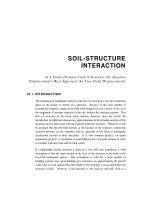
CHAPTER 1 INTRODUCTION
Buried conduits existed in prehistory when caves
were protective habitat, and ganats (tunnels back
under mountains) were dug for water. The value of
pipes is found in life forms. As life evolved, the
more complex the organism, the more vital and
complex were the piping systems.

In a phenomenon as complex as the soil-structure
interaction of buried pipes, all three sources must be
utilized.
There are too many variables; the
interaction is too complex (statically indeterminate to
the infinite degree); and the properties of soil are too
imprecise to rely on any one source of information.

The earthworm lives in buried tunnels. His is a
higher order of life than the amoeba because he has
developed a gut — a pipe — for food processing
and waste disposal.

Buried structures have been in use from antiquity.
The ancients had only experience as a source of
knowledge. Nevertheless, many of their catacombs,
ganats, sewers, etc., are still in existence. But they
are neither efficient nor economical, nor do we have

any idea as to how many failed before artisans
learned how to construct them.

The Hominid, a higher order of life than the
earthworm, is a magnificent piping plant. The
human piping system comprises vacuum pipes,
pressure pipes, rigid pipes, flexible pipes — all
grown into place in such a way that flow is optimum
and stresses are minimum in the pipes and between
the pipes and the materials in which they are buried.
Consider a community. A termite hill contains an
intricate maze of pipes for transportation, ventilation,
and habitation. But, despite its elegance, the termite
piping system can't compare with the piping systems
of a community of people. The average city dweller
takes for granted the services provided by city piping
systems, and refuses to contemplate the
consequences if services were disrupted. Cities can
be made better only to the extent that piping systems
are made better. Improvement is slow because
buried pipes are out-of-sight, and, therefore, out-ofmind to sources of funding for the infrastructure.
Engineering design requires knowledge of: 1.
performance, and 2. limits of performance. Three
general sources of knowledge are:
SOURCES OF KNOWLEDGE
Experience
Experimentation
Principles

©2000 CRC Press LLC

(Pragmatism)
(Empiricism)
(Rationalism)

The other two sources of knowledge are recent.
Experimentation and principles required the
development of soil mechanics in the twentieth
century. Both experience and experimentation are
needed to verify principles, but principles are the
basic tools for design of buried pipes.
Complex soil-structure interactions are still analyzed
by experimentation. But even experimentation is
most effective when based on principles — i.e.,
principles of experimentation.
This text is a compendium of basic principles proven
to be useful in structural design of buried pipes.
Because the primary objective is design, the first
principle is the principle of design.

DESIGN OF BURIED PIPES
To design a buried pipe is to devise plans and
specifications for the pipe-soil system such that
performance does not reach the limits of
performance.
Any performance requirement is
equated to its limit divided by a safety factor, sf, i.e.:


Figure 1-1 Bar graph of maximum peak daily pressures in a water supply pipeline over a period of 1002 days

with its corresponding normal distribution curve shown directly below the bar graph.

©2000 CRC Press LLC


Performance =

Performance Limit
Safety Factor

Examples:
Stress = Strength/sf
Deformation = Deformation Limit/sf
Expenditures = Income/sf; etc.
If performance were exactly equal to the performance
limit, half of all installations would fail. A safety
factor, sf, is required. Designers must allow for
imperfections such as less-than-perfect construction,
overloads, flawed materials, etc. At present, safety
factors are experience factors. Future safety factors
must include probability of failure, and the cost of
failure — including risk and liability. Until then, a
safety factor of two is often used.
In order to find probability of failure, enough failures
are needed to calculate the standard deviation of
normal distribution of data.

NORMAL DISTRIBUTION
Normal distribution is a plot of many measurements
(observations) of a quantity with coordinates x and y,

where, see Figure 1-1,
x = abscissa = measurement of the quantity,
y = ordinate = number of measurements in any given
x-slot. A slot contains all measurements that are
closer to the given x than to the next higher x or the
next lower x. On the bar graph of data Figure 1-1, if
x = 680 kPa, the 680-slot contains all of x-values
from 675 to 685 kPa.
x)
x
n
w
P

= the average of all measurements,
= 3yx/3y,
= total number of measurements = Ey,
= deviation, w = x - x) ,
= probability that measurement will fall
between ±w,
Pe = probability that a measurement will exceed
the failure level of xe (or fall below a
minimum level of xe ),

©2000 CRC Press LLC

s

=

standard deviation = deviation within which
68.26 percent of all measurements fall (Ps =
68.26%).

P is the ratio of area within +w and the total area.
Knowing w/x, P can be found from Table 1.1. The
standard deviation s is important because: l. it is a
basis for comparing the precision of sets of
measurements, and 2. it can be calculated from
actual measurements; i.e.,
s = %3yw2/(n-1)
Standard deviation s is the horizontal radius of
gyration of area under the normal distribution curve
measured from the centroidal y axis. s is a deviation
of x with the same dimensions as x and w. An
important dimensionless variable (pi-term) is w/s.
Values are listed in Table 1-1. Because probability
P is the ratio of area within ±w and the total area, it
is also a dimensionless pi-term. If the standard
deviation can be calculated from test data, the
probability that any measurement x will fall within
±w from the average, can be read from Table 1-1.
Likewise the probability of a failure, Pe , either
greater than an upper limit xe or less than a lower
limit, xe , can be read from the table. The deviation
of failure is needed; i.e., we = x e - x) . Because pipesoil interaction is imprecise (large standard
deviation), it is prudent to design for a probability of
success of 90% (10% probability of failure) and to
include a safety factor. Probability analysis can be
accomplished conveniently by a tabular solution as

shown in the following example.
Example
The bursting pressure in a particular type of pipe has
been tested 24 times with data shown in Table 1-2.
What is the probability that an internal pressure of
0.8 MPa (120 psi or 0.8 MN/m2) will burst the pipe?
x = test pressure (MN/m2) at bursting
y = number of tests at each x
n = Gy = total number of tests


Table 1-1 Probability P as a function of w/s that a value of x will fall within +w, and probability Pe a s a
function of we /s that a value of x will fall outside of +w e on either the +w e or the -w e .
w e /s
____
0.0
0.1
0.2
0.3
0.4

P
(%)
0.0
8.0
15.9
23.6
31.1

Pe

(%)
50.0
46.0
42.1
38.2
34.5

w e /s
____
1.5
1.6
1.7
1.8
1.9

P
(%)
86.64
89.04
91.08
92.82
94.26

Pe
(%)
6.68
5.48
4.46
3.59
2.87

0.5
0.6
0.6745
0.7

38.3
45.1
50.0
51.6

30.9
27.4
25.0
24.2

2.0
2.1
2.2
2.3

95.44
96.42
97.22
97.86

2.28
1.79
1.39
1.07

0.8
0.9

57.6
63.2

21.2
18.4

2.4
2.5

98.36 0.82
98.76 0.62

1.0
1.1
1.2
1.3
1.4

68.26
72.9
78.0
80.6
83.8

15.9
13.6

11.5
9.7
8.1

2.6
2.7
2.8
2.9
3.0

99.06
99.30
99.48
99.62
99.74

0.47
0.35
0.26
0.19
0.135

Table 1-2 Pressure data from identical pipes tested to failure by internal bursting pressure, and a tabular
solution of the average bursting pressure and its standard deviation.
x
(Mpa)*
0.9
1.0
1.1
1.2

1.3
1.4
Sums

y
xy
_ (MPa)
2 1.8
7 7.0
8 8.8
4 4.8
2 2.6
1 1.4
24 26.4
n Σxy

w
(MPa)
-0.2
-0.1
0.0
+0.1
+0.2
+0.3

yw
(MPa)
-0.4
-0.7
0.0

+0.4
+0.4
+0.3

yw 2
(MPa) 2
0.08
0.07
0.00
0.04
0.08
0.09
0.36
Σyw 2

x = Sxy/n = 1.1 MPa
s = [ Syw 2/(n-1)] = 0.125
*MPa is megapascal of pressure where a Pascal is N/m2; i.e., a megapascal is a million Newtons of forc e
per square meter of area. A Newton = 0.2248 lb. A square meter = 10.76 square ft.

©2000 CRC Press LLC


From the data of Table 1-2,
_

x

=

Σxy/Sy = 26.4/24 = 1.1

s

=

\

w

=

_
x - x, so

/Syw /(n-1) = \/0.36/23
2

= 0.125

w e = (0.8 - 1.1) = -0.30 MN/m2
= deviation to failure pressure
w e/s =

0.30/0.125 = 2.4.

From Table 1-1, interpolating, Pe= 0.82%.
The probability that a pipe will fail by bursting
pressure less than 0.80 MN/m2 is Pe = 0.82 % or
one out of every 122 pipe sections. Cost accounting

of failures then follows.
The probability that the strength of any pipe section
will fall within a deviation of w e = +0.3 MN/m2 is P
= 98.36%. It is noteworthy that P + 2Pe = 100%.
From probability data, the standard deviation can be
calculated. From standard deviation, the zone of +w
can be found within which 90% of all measurements
fall. In this case w/s = w/0.125 for which P = 90%.
From Table 1-1, interpolating for P = 90%, w/s =
1.64%, and w = 0.206 MPa at 90% probability.
Errors (three classes)
Mistake = blunder —
Remedies: double-check, repeat.
Accuracy = nearness to truth —
Remedies: calibrate, repair, correct.
Precision = degree of refinement —
Remedies: normal distribution, safety factor.

PERFORMANCE
Performance in soil-structure interaction is
deformation as a function of loads, geometry, and
properties of materials. Some deformations can be
written in the form of equations from principles of

©2000 CRC Press LLC

soil mechanics.
The remainders involve such
complex soil-structure interactions that the
interrelationships must be found from experience or

experimentation. It is advantageous to write the
relationships in terms of dimensionless pi-terms. See
Appendix C. Pi-terms that have proven to be useful
are given names such as Reynold's number in fluid
flow in conduits, Mach number in gas flow, influence
numbers, stability numbers, etc.
Pi-terms are independent, dimensionless groups of
fundamental variables that are used instead of the
original fundamental variables in analysis or
experimentation. The fundamental variables are
combined into pi-terms by a simple process in which
three characteristic s of pi-terms must be satisfied.
The starting point is a complete set of pertinent
fundamental variables. This requires familiarity with
the phenomenon. The variables in the set must be
interdependent, but no subset of variables can be
interdependent. For example, force f, mass m, and
acceleration a, could not be three of the fundamental
variables in a phenomenon which includes other
variables because these three are not independent;
i.e., f = ma. Only two of the three would be
included as fundamental variables.
Once the
equation of performance is known, the deviation, w,
can be found. Suppose r = f(x,y,z,...), then w r2 =
Mrx2
w x2 + Mry 2w y 2 + ... where w is a deviation at the
same given probability for all variables, such as
standard deviation with probability of 68%; mrx is the
tangent to the r-x curve and wx is the deviation at a

given value of x. The other variables are treated in
the same way.

CHARACTERISTICS OF PI-TERMS
1. Number of pi-terms = (number of fundamental
variables) minus (number of basic dimensions).
2.

All pi-terms are dimensionless.

3.
Each pi-term is independent. Independence is
assured if each pi-term contains a fundamental
variable not contained in any other pi-term.


Figure 1-2 Plot of experimental data for the dimensionless pi-terms (P'/S) and (t/D) used to find the equation
for bursting pressure P' in plain pipe. Plain (or bare) pipe has smooth cylindrical surfaces with constant wall
thickness — not corrugated or ribbed or reinforced.

Figure 1-3 Performance limits of the soil showing how settlement of the soil backfill leaves a dip in the
surface over a flexible (deformed) pipe and a hump and crack in the surface over a rigid (undeformed) pipe.

©2000 CRC Press LLC


Pi-terms have two distinct advantages: fewer
variables to relate, and the elimination of size effect.
The required number of pi-terms is less than the
number of fundamental variables by the number of

basic dimensions.
Because pi-terms are
dimensionless, they have no feel for size (or any
dimension) and can be investigated by model study.
Once pi-terms have been determined, their
interrelationships can be found either by theory
(principles) or by experimentation. The results apply
generally because the pi-terms are dimensionless.
Following is an example of a well-designed
experiment.

small scale model study are plotted in Figure 1-2.
The plot of data appears to be linear. Only the last
point to the right may deviate. Apparently the pipe
is no longer thin-wall. So the thin-wall designation
only applies if t/D< 0.1. The equation of the plot is
the equation of a straight line, y = mx + b where y is
the ordinate, x is the abscissa, m is the slope, and b
is the y-intercept at x = 0. For the case above,
(P'/S) = 2(t/D), from which, solving for bursting
pressure,
P = 2S/(D/t)
This important equation is derived by theoretical
principles under "Internal Pressure," Chapter 2.

Example
Using experimental techniques, find the equation for
internal bursting pressure, P', for a thin-wall pipe.
Start by writing the set of pertinent fundamental
variables together with their basic dimensions, force

F and length L.

Fundamental Variables
P'
t
D
S

=
=
=
=

internal pressure
wall thickness
inside diameter of ring
yield strength of the
pipe wall material

Basic
Dimensions
FL-2
L
L
FL-2

These four fundamental variables can be reduced to
two pi-terms such as (P'/S) and (t/D). The pi-terms
were written by inspection keeping in mind the three
characteristics of pi-terms. The number of pi-terms

is the number of fundamental variables, 4, minus the
number of basic dimensions, 2, i.e., F and L. The
two pi-terms are dimensionless.
Both are
independent because each contains a fundamental
variable not contained in the other. Conditions for
bursting can be investigated by relating only two
variables, the pi-terms, rather than interrelating the
original four fundamental variables. Moreover, the
investigation can be performed on pipes of any
convenient size because the pi-terms are
dimensionless. Test results of a
©2000 CRC Press LLC

PERFORMANCE LIMITS
Performance limit for a buried pipe is basically a
deformation rather than a stress. In some cases it is
possible to relate a deformation limit to a stress
(such as the stress at which a crack opens), but
such a relationship only accommodates the designer
for whom the stress theory of failure is familiar. In
reality, performance limit is that deformation beyond
which the pipe-soil system can no longer serve the
purpose for which it was intended.
The
performance limit could be a deformation in the soil,
such as a dip or hump or crack in the soil surface
over the pipe, if such a deformation is unacceptable.
The dip or hump would depend on the relative
settlement of the soil directly over the pipe and the

soil on either side. See Figure 1-3.
But more often, the performance limit is excessive
deformation of the pipe whic h could cause leaks or
could restrict flow capacity. If the pipe collapses
due to internal vacuum or external hydrostatic
pressure, the restriction of flow is obvious. If, on the
other hand, the deformation of the ring is slightly outof-round, the restriction to flow is usually not
significant. For example, if the pipe cross section
deflects into an ellipse such that the decrease of the
minor diameter is 10% of the original circular
diameter, the decrease in cross-sectional area is only
1%.


Figure 1-4 Typical performance limits of buried pipe rings due to external soil pressure.
©2000 CRC Press LLC


The more common performance limit for the pipe is
that deformation beyond which the pipe cannot resist
any increase in load. The obvious case is bursting of
the pipe due to internal pressure. Less obvious and
more complicated is the deformation due to external
soil pressure. Typical examples of performance
limits for the pipe are shown in Figure 1-4. These
performance limits do not imply collapse or failure.
The soil generally picks up any increase in load by
arching action over the pipe, thus protecting the pipe
from total collapse. The pipe may even continue to
serve, but most engineers would prefer not to

depend on soil alone to maintain the conduit cross
section. This condition is considered to be a
performance limit. The pipe is designed to withstand
all external pressures. Any contribution of the soil
toward withstanding external pressure by arching
action is just that much greater margin of safety.
The soil does contribute soil strength. On inspection,
many buried pipes have been found in service even
though the pipe itself has "failed." The soil holds
broken clay pipes in shape for continued service.
The inverts of steel culverts have been corroded or
eroded away without failure. Cast iron bells have
been found cracked. Cracked concrete pipes are
still in service, etc. The mitigating factor is the
embedment soil which supports the conduit.

the structural design of the pipe can proceed in six
steps as follows.

STEPS IN THE STRUCTURAL DESIGN OF
BURIED PIPES
In order of importance:
1. Resistance to internal pressure, i.e., strength of
materials and minimum wall thickness;
2. Resistance to transportation and installation;
3. Resistance to external pressure and internal
vacuum, i.e., ring stiffness and soil strength;
4. Ring deflection, i.e., ring stiffness and soil
stiffness;
5. Longitudinal stresses and deflections;

6. Miscellaneous concerns such as flotation of the
pipe, construction loads, appurtenances, ins tallation
techniques, soil availability, etc.

A reasonable sequence in the design of buried pipes
is the following:

Environment, aesthetics, risks, and costs must be
considered. Public relations and social impact
cannot be ignored. However, this text deals only
with structural design of the buried pipe.

1. Plans for delivery of the product (distances,
elevations, quantities, and pressures),

PROBLEMS

2. Hydraulic design of pipe sizes, materials,
3. Structural requirements and design of possible
alternatives,
4. Appurtenances for the alternatives,
5. Economic analysis, costs of alternatives,
6. Revision and iteration of steps 3 to 5,
7. Selection of optimum system.
With pipe sizes, pressures, elevations, etc., known

©2000 CRC Press LLC

1-1 Fluid pressure in a pipe is 14 inches of mercury
as measured by a manometer. Find pressure in

pounds per square inch (psi) and in Pascals
(Newtons per square meter)? Specific gravity of
mercury is 13.546.
(6.85 psi)(47.2 kPa)
1-2 A 100 cc laboratory sample of soil weighs 187.4
grams mass. What is the unit weight of the soil in
pounds per cubic ft?
(117 pcf)
1-3 Verify the standard deviation of Figure 1-1.
(s = 27.8 kPa)


1-4 From Figure 1-1, what is the probability that
any maximum daily pressure will exceed 784.5
kPa?
(Pe = 0.62%)
1-5 Figure 1-5 shows bar graph for internal vacuum
at collapse of a sample of 58 thin-walled plastic
pipes.
x = collapse pressure in Pascals, Pa.
(Least increment is 5 Pa.)
y = number that collapsed at each value of x.
(a) What is the average vacuum at collapse?
(75.0 Pa)
(b) What is the standard deviation?
(c) What is the probable error?

(8.38 Pa)
(+5.65 Pa)

1-6 Eleven 30 inch ID, non-reinforced concrete
pipes, Class 1, were tested in three-edge-bearing
(TEB) test with results as follows:
x = ultimate load in pounds per lineal ft
x
w
w2
(lb/ft)
(lb/ft)
3562
3125
4375
3438
4188
3688
3750
4188
4125
3625
2938
(a) What is the average load, x, at failure?
(x = 3727.5 lb/ft)
(b) What is the standard deviation?
(s = 459.5 lb/ft)
(c) What is the probability that the load, x, at failure
is less than the minimum specified strength of 3000
lb/ft (pounds per linear ft)?
(Pe = 5.68%)

©2000 CRC Press LLC

Figure 1-5 Bar graphs of internal vacuum at collapse
of thin-walled plastic pipes.

1-7 Fiberglass reinforced plastic (FRP) tanks were
designed for a vacuum of 4 inches of mercury
(4inHg). They were tested by internal vacuum for
which the normal distribution of the results is shown
as Series A in Figure 1-6. Two of 79 tanks failed at
less than 4inHg. In Series B, the percent of
fiberglas was increased. The normal distribution
curve has the same shape as Series A, but is shifted
1inHg to the right. What is the predicted probability
of failure of Series B at or below 4 in Hg?
(Pe = 0.17 % or one tank in every 590)
1-8 What is the probability that the vertical ring
deflection d = y/D of a buried culvert will exceed
10% if the following measurements were made on
23 culverts under identical conditions?
Measured values of d (%)
6 9 6 6 5 6
8 5 4 6 7 7
3 6 7 5 4 5
6 7 8 7 5
(0.24 %)
1-9 The pipe stiffness is measured for many samples
of a particular plastic pipe. the average is 24 with a
standard deviation of 3.
a) What is the probability that the pipe stiffness will
be less than 20?

(Pe = 9.17 %)


b) What standard deviation is required if the
probability of a stiffness less than 20 is to be
reduced to half its present value; i.e., less than
4.585%?
(s = 2.37)

1-10 A sidehill slope of cohesionless soil dips at
angle 2. Write pi-terms for critical slope when
saturated.
1-11 Design a physical model for problem 1-10.

Figure 1-6 Normal distribution diagrams for fiberglass tanks designed for 4inHg vacuum.
©2000 CRC Press LLC