Springer pattern recognition concepts methods and applications (2001) 3540422978 irb

J. P. Marques de Sa

Pattern Recoanition
Concepts, Methods and Applications

With 197 Figures

Springer


To
my wife Wiesje
and our son Carlos,
lovingly.


Preface

Pattern recognition currently comprises a vast body of methods supporting the
development of numerous applications in many different areas of activity. The
generally recognized relevance of pattern recognition methods and techniques lies,
for the most part, in the general trend o r "intelligent" task emulation, which has
definitely pervaded our daily life. Robot assisted manufacture, medical diagnostic
systems, forecast of economic variables, exploration of Earth's resources, and
analysis of satellite data are just a few examples of activity fields where this trend
applies. The pervasiveness of pattern recognition has boosted the number of taskspecific methodologies and enriched the number of links with other disciplines. As
counterbalance to this dispersive tendency there have been, more recently, new
theoretical developments that are bridging together many of the classical pattern
recognition methods and presenting a new perspective of their links and inner
workings.

This book has its origin in an introductory course on pattern recognition taught
at the Electrical and Computer Engineering Department, Oporto University. From
the initial core of this course, the book grew with the intent of presenting a
comprehensive and articulated view of pattern recognition methods combined with
the intent of clarifying practical issucs with the aid ofexarnples and applications to
real-life data. The book is primarily addressed to undergraduate and graduate
students attending pattern recognition courses of engineering and computer science
curricula. In addition to engineers or applied mathematicians, it is also common for
professionals and researchers from other areas of activity to apply pattern
recognition methods, e.g. physicians, biologists, geologists and economists. The
book includes real-life applications and presents matters in a way that reflects a
concern for making them interesting to a large audience, namely to non-engineers
who need to apply pattern recognition techniques in their own work, or who
happen to be involved in interdisciplinary projects employing such techniques.
Pattern recognition involves mathematical models of objects described by their
features or attributes. It also involves operations on abstract representations of what
is meant by our common sense idea of similarity or proximity among objects. The
mathematical formalisms, models and operations used, depend on the type of
problem we need to solve. In this sense, pattern recognition is "mathematics put
into action". Teaching pattern recognition without getting the feedback and insight
provided by practical examples and applications is a quite limited experience, to
say the least. We have, therefore, provided a CD with the book, including real-life
data that the reader can use to practice the taught methods or simply to follow the
explained examples. The software tools used in the book are quite popular, in thc
academic environment and elsewhere, so closely following the examples and


.. .

VI~I

Preface

checking the presented results should not constitute a major difficulty. The CD also
includes a set of complementary software tools for those topics where the
availability of such tools is definitely a problem. Therefore, from the beginning of
the book, the reader should be able to follow the taught methods with the guidance
of practical applications, without having to do any programming, and concentrate
solely on the correct application of the learned concepts.
The main organization of the book is quite classical. Chapter 1 presents the
basic notions of pattern recognition, including the three main approaches
(statistical, neural networks and structural) and important practical issues. Chapter
2 discusses the discrimination of patterns with decision functions and
representation issues in the feature space. Chapter 3 describes data clustering and
dimensional reduction techniques. Chapter 4 explains the statistical-based methods,
either using distribution models or not. The feature selection and classifier
evaluation topics are also explained. Chapter 5 describes the neural network
approach and presents its main paradigms. The network evaluation and complexity
issues deserve special attention, both in classification and in regression tasks.
Chapter 6 explains the structural analysis methods, including both syntactic and
non-syntactic approaches. Description of the datasets and the software tools
included in the CD are presented in Appendices A and B.
Links among the several topics inside each chapter, as well as across chapters,
are clarified whenever appropriate, and more recent topics, such as support vector
machines, data mining and the use of neural networks in structural matching, are
included. Also, topics with great practical importance, such as the dimensionality
ratio issue, are presented in detail and with reference to recent findings.
All pattern recognition methods described in the book start with a presentation
of the concepts involved. These are clarified with simple examples and adequate
illustrations. The mathematics involved in the concepts and the description of the

methods is explained with a concern for keeping the notation cluttering to a
minimum and using a consistent symbology. When the methods have been
sufficiently explained, they are applied to real-life data in order to obtain the
needed grasp of the important practical issues.
Starting with chapter 2, every chapter includes a set of exercises at the end. A
large proportion of these exercises use the datasets supplied with the book, and
constitute computer experiments typical of a pattern recognition design task. Other
exercises are intended to broaden the understanding of the presented examples,
testing the level of the reader's comprehension.
Some background in probability and statistics, linear algebra and discrete
mathematics is needed for full understanding of the taught matters. In particular,
concerning statistics, it is assumed that the reader is conversant with the main
concepts and methods involved in statistical inference tests.
All chapters include a list of bibliographic references that support all
explanations presented and constitute, in some cases, pointers for further reading.
References to background subjects are also included, namely in the area of
statistics.
The CD datasets and tools are for the Microsoft Windows system (95 and
beyond). Many of these datasets and tools are developed in Microsoft Excel and it
should not be a problem to run them in any of the Microsoft Windows versions.


Preface

ix

The other tools require an installation following the standard Microsoft Windows
procedure. The description of these tools is given in Appendix B. With these
descriptions and the examples included in the text, the reader should not have, in
principle, any particular difficulty in using them.

Acknowledgements
In the preparation of this book I have received support and encouragement from
several persons. My foremost acknowledgement of deep gratitude goes to
Professor Willem van Meurs, researcher at the Biomedical Engineering Research
Center and Professor at the Applied Mathematics Department, both of the Oporto
University, who gave me invaluable support by reviewing the text and offering
many stimulating comments. The datasets used in the book include contributions
from several people: Professor C. Abreu Lima, Professor AurClio Campilho,
Professor Joiio Bernardes, Professor Joaquim Gois, Professor Jorge Barbosa, Dr.
Jacques Jossinet, Dr. Diogo A. Campos, Dr. Ana Matos and J050 Ribeiro. The
software tools included in the CD have contributions from Eng. A. Garrido, Dr.
Carlos Felgueiras, Eng. F. Sousa, Nuno AndrC and Paulo Sousa. All these
contributions of datasets and softwarc tools are acknowledged in Appendices A
and B, respectively. Professor Pimenta Monteiro helped me review the structural
pattern recognition topics. Eng. Fernando Sereno helped me with the support
vector machine experiments and with the review of the neural networks chapter.
Joiio Ribeiro helped me with the collection and interpretation of economics data.
My deepest thanks to all of them. Finally, my thanks also to Jacqueline Wilson,
who performed a thorough review of the formal aspects of the book.
Joaquim P. Marques de Sa
May, 2001
Oporto University, Portugal


Contents

Preface ....................................................................................................... vii

Contents .....................................................................................................xi

..
Symbols and Abbreviations ................................................................. xvll

1

Basic Notions ..................................................................................... 1
Object Recognition ....................................................................... 1
Pattern Similarity and PR Tasks ...................................................2
1.2.1 Classification Tasks ......................................................... 3
1.2.2
Regression Tasks ........................................................6
1.2.3 Description Tasks ............................................................8
Classes, Patterns and Features ................................................... 9
1.3
1.4
PRApproaches .......................................................................... 13
1.4.1 Data Clustering..............................................................14
1.4.2 Statistical Classification................................................. 14
1.4.3 Neural Networks ............................................................15
1.4.4 Structural PR .................................................................16
1.5
PR Project ..................................................................................16
15 . 1 Project Tasks ................................................................. 16
15 . 2 Training and Testing .................................................. 18
1.5.3 PR Software .................................................................. 18
Bibliography............................................................................................ 20

1.1
1.2

2

Pattern Discrimination ....................................................................... 21
2.1

2.2
2.3

Decision Regions and Functions................................................21
2.1 .1 Generalized Decision Functions ...................................23
2.1.2 Hyperplane Separability ................................................ 26
Feature Space Metrics ...............................................................
29
33
The Covariance Matrix ...............................................................


xi i

Contents

Principal Components ............................................................... 39
Feature Assessment ..................................................................41
2.5.1 Graphic Inspection ........................................................42
2.5.2 Distribution Model Assessment .....................................43
2.5.3
Statistical Inference Tests ............................................. 44
2.6
The Dimensionality Ratio Problem ............................................. 46

Bibliography............................................................................................49
Exercises ................................................................................................49

2.4
2.5

3

Data Clustering..................................................................................53
Unsupervised Classification .......................................................
53
The Standardization Issue......................................................
55
Tree Clustering ...........................................................................
58
3.3.1 Linkage Rules ................................................................
60
3.3.2 Tree Clustering Experiments.........................................
63
3.4
Dimensional Reduction ..............................................................
65
3.5
K-Means Clustering ....................................................................
70
73
3.6
Cluster Validation .......................................................................
Bibliography............................................................................................
76

77
Exercises ................................................................................................
3.1
3.2
3.3

4

Statistical Classification....................................................................79
Linear Discriminants...................................................................
79
4.1 .1 Minimum Distance Classifier ........................................ 79
4.1 .2 Euclidian Linear Discriminants ......................................82
4.1 .3 Mahalanobis Linear Discriminants ................................85
4.1.4
Fisher's Linear Discriminant ..........................................
88
Bayesian Classification .............................................................. 90
4.2.1 Bayes Rule for Minimum Risk .......................................
90
97
4.2.2
Normal Bayesian Classification.....................................
4.2.3 Reject Region ..............................................................
103
4.2.4
Dimensionality Ratio and Error Estimation..................105
108
Model-Free Techniques ...........................................................
4.3.1 The Parzen Window Method .......................................110

4.3.2 The K-Nearest Neighbours Method ............................113
4.3.3 The ROC Curve ...........................................................116
Feature Selection .....................................................................
121
Classifier Evaluation.................................................................
126
Tree Classifiers ........................................................................
130
4.6.1
Decision Trees and Tables ..........................................
130
4.6.2 Automatic Generation of Tree Classifiers ................... 136


Contents

...

X~II

4.7
Statistical Classifiers in Data Mining ........................................ 138
Bibliography..........................................................................................
140
Exercises ..............................................................................................
142

5

Neural Networks ...............................................................................147

LMS Adjusted Discriminants ....................................................
147
Activation Functions ................................................................. 155
The Perceptron Concept ..........................................................159
Neural Network Types ..............................................................167
Multi-Layer Perceptrons ...........................................................171
5.5.1 The Back-PropagationAlgorithm ................................ 172
5.5.2 Practical aspects ......................................................... 175
5.5.3 Time Series ...............................................................1 8 1
Performance of Neural Networks ............................................. 184
5.6.1 Error Measures............................................................ 184
5.6.2 The Hessian Matrix .....................................................186
5.6.3 Bias and Variance in NN Design .................................189
5.6.4 Network Complexity ....................................................
192
5.6.5 Risk Minimization ........................................................ 199
201
Approximation Methods in NN Training ...................................
.................................
5.7.1 The Conjugate-Gradient Method
202
5.7.2 The Levenberg-Marquardt Method .............................205
207
Genetic Algorithms in NN Training ...........................................
Radial Basis Functions .............................................................212
Support Vector Machines .........................................................
215
Kohonen Networks ...................................................................
223
226

Hopfield Networks ..............................................................
Modular Neural Networks .........................................................
231
235
Neural Networks in Data Mining...............................................
Bibliography..........................................................................................
237
Exercises ..............................................................................................
239

6

Structural Pattern Recognition .......................................................
243
6.1
6.2

6.3

Pattern Primitives .....................................................................243
6.1 . 1 Signal Primitives ..........................................................243
6.1 .2 Image Primitives ..........................................................
245
Structural Representations.......................................................247
6.2.1 Strings .........................................................................247
6.2.2 Graphs .........................................................................
248
6.2.3 Trees ...........................................................................
249
Syntactic Analysis ................................................................... 2 5 0

6.3.1 String Grammars ......................................................... 250
6.3.2 Picture Description Language ..................................... 253
6.3.3 Grammar Types .......................................................... 255
6.3.4 Finite-State Automata .................................................. 257
6.3.5 Attributed Grammars ................................................... 260
6.3.6 Stochastic Grammars .................................................. 261
6.3.7 Grammatical Inference ................................................ 264
6.4
Structural Matching ..................................................................265
6.4.1 String Matching ........................................................... 265
6.4.2
Probabilistic Relaxation Matching ............................... 271
6.4.3 Discrete Relaxation Matching...................................... 274
6.4.4 Relaxation Using Hopfield Networks ........................... 275
6.4.5 Graph and Tree Matching ...........................................279
Bibliography ..........................................................................................283
Exercises .............................................................................................. 285

Appendix A .
CD Datasets .................................................................. 291
Breast Tissue ............................................................................ 291
Clusters .................................................................................... 292
Cork Stoppers........................................................................... 292
Crimes ...................................................................................... 293
Cardiotocographic Data............................................................ 293
Electrocardiograms .................................................................. 294
Foetal Heart Rate Signals ........................................................ 295
FHR-Apgar ............................................................................... 295

Firms ......................................................................................... 296
Foetal Weight ........................................................................... 296
Food ......................................................................................... 297
Fruits.........................................................................................297
Impulses on Noise ....................................................................
297
MLP Sets ..................................................................................298
Norm2c2d .................................................................................298
Rocks ........................................................................................ 299
Stock Exchange ....................................................................... 299
Tanks ........................................................................................ 300
Weather ....................................................................................300

Appendix B .
CD Tools ........................................................................301
B.l
B.2
B.3

Adaptive Filtering ......................................................................301
Density Estimation.................................................................... 301
Design Set Size ........................................................................302


Contents

8.4
B.5
B.6
B.7

B.8
B.9
B.10

Error Energy .............................................................................
Genetic Neural Networks .........................................................
Hopfield network .......................................................................
k-NNBounds ............................................................................
k-NN Classification ...................................................................
Perceptron ................................................................................
Syntactic Analysis ....................................................................

xv

303
304
306
308
308
309
309

Appendix C - Orthonormal Transformation ......................................... 311

Index..................................................................................................... 315


Symbols and Abbreviations

Global Symbols

number of features or primitives
number of classes or clusters
number of patterns
number of weights
class or cluster i, i = l , ... , c
number of patterns of class or cluster mi
weight i
bias
approximation error
pattern set
class set

Mathematical Symbols
variable
value of x at iteration r
i-th component of vector or string x
i-th component of vector xk
vector (column) or string
transpose vector (row)
vector x increment
inner product of x and y
i-th row, j-th column element of matrix A
matrix
transpose of matrix A
inverse of matrix A
determinant of matrix A
pseudo inverse of matrix A
identity matrix
factorial of k, k!= k(k-l)(k-2) ...2.1
combinations of n elements taken k at a time

derivative of E relative to w evaluated at w*


xviii

Svrnbols

function g evaluated at x
error function
natural logarithm function
logarithm in base 2 function
sign function
real numbers set
learning rate
eigenvalue i
null string
absolute value of x
norm
implies
converges to
produces

Statistical Symbols
sample mean
sample standard deviation
sample mean vector
sample covariance matrix
mean vector
covariance matrix
expected value of x

expected value of x given y (conditional expectation)
normal distribution with mean m and standard deviation s
discrete probability of random vector x
discrete conditional probability of wj given x
probability density function p evaluated at x
conditional probability density function p evaluated at x given
probability of ~nisclassification(error)
estimate of Pe
probability of correct classification

Abbreviations
CAM
CART
ECG
ERM

Content Addressed Memory
Classification And Regression Trees
Electrocardiogram
Empirical Risk Minimization

LO,


ERM
FHR
IPS
KFM
k-NN
ISODATA

LMS
MLP
PAC
pdf
PDL
PR
RBF
RMS
ROC
S RM
SVM
UPGMA
UWGMA
VC
XOR

Empirical Risk Minimization
Foetal Heart Rate
Intelligent Problem Solver (Stutisticu)
Kohonen's Feature Map
k - Nearest Neighbours
Iterative Self-organizing Data Analysis Technique
Least Mean Square
Multi-layer perceptron
Probably Approxi~natelyCorrect
Probability Density Function
Picture Description 1,anguage
Pattern Recognition
Radial Basis Functions
Root Mean Square

Receiver Operating Characteristic
Structural Risk Minimization
Support Vector Machine
Un-weighted Pair-Group Method using arithmetic Averages
Un-weighted Within-Group Method using arithmetic Averages
Vapnik-Chervonenkis (dimension)
Exclusive OR

Tradenames
Mallab
Excel
SPSS
Statjstica
Windows

The Mathworks, lnc.
Microsoft Corporation
SPSS, Inc.
Statsoft, Inc.
Microsoft Corporation


1 Basic Notions

1.1 Object Recognition
Object recognition is a task performed daily by living beings and is inherent to
their ability and necessity to deal with the environment. It is performed in the most
varied circumstances - navigation towards food sources, migration, identification
of predators, identification of mates, etc. - with remarkable efficiency. Recognizing
objects is considered here in a broad cognitive sense and may consist of a very

simple task, like when a micro-organism flees from an environment with
inadequate pH, or refer to tasks demanding non-trivial qualities of inference,
description and interpretation, for instance when a human has to fetch a pair of
scissors from the second drawer of a cupboard, counting from below.
The development of methods capable of emulating the most varied forms of
object recognition has evolved along with the need for building "intelligent"
automated systems, the main trend of today's technology in industry and in other
fields of activity as well. ln these systems objects are represented in a suitable way
for the type of processing they are subject to. Such representations are called
patterns. In what follows we use the words object and pattern interchangeably with
similar meaning.
Pattern Recognition (PR) is the scientific discipline dealing with methods for
object description and classikication. Since the early times of computing the design
and implementation of algorithms emulating the human ability to describe and
classify objects has been found a most intriguing and challenging task. Pattern
recognition is therefore a fertile area of research, with multiple links to many other
disciplines, involving professionals from several areas.
Applications of pattern recognition systems and techniques are numerous and
cover a broad scope of activities. We enumerate only a few examples referring to
several professional activities:

Agriculture:
Crop analysis
Soil evaluation
Astronomy:
Analysis of telescopic images
Automated spectroscopy
Biology:
Automated cytology
Properties of chromosomes

Genetic studies


2

I Basic Notions

Civil administration:
Traffic analysis and control
Assessment of urban growth
Economy:
Stocks exchange forecast
Analysis of entrepreneurial performance
Engineering:
Fault detection in manufactured products
Character recognition
Speech recognition
Automatic navigation systen~s
Pollution analysis
Geology:
Classification of rocks
Estimation of mining resources
Analysis of geo-resources using satellite images
Seismic analysis
Medicine:
Analysis of electrocardiograms
Analysis of electroencephalograms
Analysis of medical images
Military:
Analysis of aerial photography

Detection and classification of radar and sonar signals
Automatic target recognition
Security:
Identification of fingerprints
Surveillance and alarm systems
As can be inferred from the above examples the pattern.; to be analysed and
recognized can be signals (e.g. e1ectrc)cardiographic signals), images (e.g. aerial
photos) or plain tables of values (e.g. stock exchange rates).

1.2 Pattern Similarity and PR Tasks
A fundamental notion in pattern recognition, independent of whatever approach we
may follow, is the notion of .similarity. We recognize two objects as being similar
because they have similarly valued common attributes. Often the similarity is
stated in a more abstract sense, not among objects but between an object and a
target concept. For instance, we recognise an object as being an apple because it
corresponds, in its features. to the idealized image, concept or prototype, we may
have of an apple, i.e., the object is similar to that concept and dissimilar from
others, for instance from an orange.


1.2 Pattern Similarity and PR Tasks

3

Assessing the similarity of patterns is strongly related to the proposed pattern
recognition task as described in the following.

1.2.1 Classification Tasks
When evaluating the similarity among objects we resort to feutures or attributes
that are of distinctive nature. Imagine that we wanted to design a system for

discriminating green apples from oranges. Figure 1.1 illustrates possible
representations of the prototypes "green apple" and "orange". In this discrimination
task we may use as obvious distinctive features the colour and the shape,
represented in an adequate way.

Figure 1.1. PossiL., :epresentations of the prototypes "green apple" and "orange".

Figure 1.2. Examples of "red apple" and "greenish orange" to be characterized by
shape and colour features.


4

1 Basic Notions

In order to obtain a numeric representation of the colour feature we may start by
splitting the image of the objects into the red-green-blue components. Next we
may, for instance, select a central region of interest in the image and compute, for
that region, the ratio of the maximum histogram locations for the red and green
components in the respective ranges (usually [O, 2551; O=no colour, 255=fuII
colour). Figure 1.3 shows the grey image corresponding to the green component of
the apple and the light intensity histogram for a rectangular region of interest. The
maximum of the histogram corresponds to 186. This means that the green intensity
value occurring most often is 186. For the red component we would obtain the
value 150. The ratio of these values is 1.24 revealing the predominance of the
green colour vs. the red colour.
In order to obtain a numeric representation of the shape feature we may, for
instance, measure the distance. away from the top, of the maximum width of the
object and normalize this distance by the height, i.e., computing xlh, with x, h
shown in Figure 1.3a. In this case, x/h=0.37. Note that we are assuming that the

objects are in a standard upright position.

Figure 1.3. (a) Grey image of the green component of the apple image; (b)
Histogram of light intensities for the rectangular region of interest shown in (a).

If we have made a sensible choice of prototypes we expect that representative
samples of green apples and ornngcs correspond to clusters of points around the
prototypes in the 2-dimensional feature space, as shown in Figure 1.4a by the
curves representing the cluster boundaries. Also, if we made a good choice of the
features, it is expected that the mentioned clusters are reasonably separated,
therefore allowing discrimination of the two classes of fruits.
The PR task of assigning an object to a class is said to be a classification task.
From a mathematical point of view i t is convenient in classification tasks to
represent a pattern by a vector, which is 2-dimensional in the present case:


1.2 Pattern Similarity and PR Tasks

5

colour
shape

For the green apple prototype we have therefore:

The points corresponding to the feature vectors of the prototypes are represented
by a square and a circle, respectively for the green apple and the orange, in Figure
1.4.
Let us consider a machine designed to separate green apples from oranges using
the described features. A piece of fruit is presented to the machine, its features are

computed and correspond to the point x (Figure 1.4a) in the colour-shape plane.
The machine, using the feature values as inputs, then has to decide if it is a green
apple or an orange. A reasonable decision is based on the Euclidian distance of the
point x from the prototypes, i.e., for the machine the similarity is a distance and in
this case it would decide "green apple". The output of the machine is in this case
any two-valued variable, e.g.. 0 corresponding to green apples and 1 corresponding
to oranges. Such a machine is called a classifier.

-

1 40

green

--

.

-,
green~ahormge

oranges
red apple

a

O23
;O

040

050

060

X~
7
4

070

Figure 1.4. (a) Green apples and oranges in the feature space; (b) A red apple
"resembling" an orange and a problematic greenish orange.

I

Imagine that our classifier receives as inputs the features of the red apple and
the greenish orange presented in Figure 1.2. The feature vectors correspond to the
points shown in Figure 1.4b. The red apple is wrongly classified as an orange since
it is much closer to the orange prototype than to the green apple prototype. This is
not a surprise since, after all, the classifier is being used for an object clearly


6

1 Basic Notions

outside its scope. As for the greenish orange its feature vector is nearly at equal
distance from both prototypes and its classification is problematic. If we use,
instead of the Euclidian distance, another distance measure that weighs more

heavily vertical deviations than horizontal deviations, the greenish orange would
also be wrongly classified.
In general practice pattern classification systems are not flawless and we may
expect errors due to several causes:
- The features used are inadequate or insufficient. For instance, the classification

of the problematic greenish orange would probably improve by using an
additional texture feature measuring the degree of surface roughness.
- The pattern
samples used to design the classifier are not sufficiently
representative. For instance, if our intention is to discriminate apples from
oranges we should have to include in the apples sample a representative variety
of apples, including the red ones as well.
- The classifier is not efficient enough in separating the classes. For instance, an
inefficient distance measure or inadequate prototypes are being used.
- There is an intrinsic overlap of the classes that no classifier can resolve.
In this book we will focus our attention on the aspects that relate to the selection
of adequate features and to the design of efficient classifiers. Concerning the initial
choice of features it is worth noting that this is more an art than a science and, as
with any art, it is improved by experimentation and practice. Besides the
appropriate choice of features and similarity measures, there are also other aspects
responsible for the high degree of classifying accuracy in humans. Aspects such as
the use of contextual information and advanced knowledge structures fall mainly in
the domain of an artificial intelligence course and will be not dealt with in this
book. Even the human recognition of objects is not always flawless and contextual
information risks classifying a greenish orange as a lemon if it lies in a basket with
lemons.
1.2.2 Regression Tasks

We consider now another type of task, directly related to the cognitive inference

process. We observe such a process when animals start a migration based on
climate changes and physiological changes of their internal biological cycles. In
daily life, inference is an important tool since it guides decision optimisation. Wellknown examples are, for instance, keeping the right distance from the vehicle
driving ahead in a road, forecasting weather conditions, predicting firm revenue of
investment and assessing loan granting based on economic variables.
Let us consider an example consisting of forecasting firm A share value in the
stock exchange market, based on past information about: the share values of firm A
and of other firms; the currency exchange rates; the interest rate. In this situation
we want to predict the value of a variable based on a sequence of past values of the
same and other variables, which in the one-day forecast situation of Figure 1.5 are:
r,, r ~rc,
, Euro-USD rate, Interest rate for 6 months.


1.2 Pattern Similarity and PR Tasks

7

As can be appreciated this time-series prediction task is an example o f a broader
class o f tasks known in mathematics as function approximation or regression /ask.
A system providing the regression solution will usually make forecasts (black
circles in Figure 1.5) somewhat deviated from the true value (curve, idem). The
difference between the predicted value and the true value, also known as target
value, constitutes a prediction error. Our aim is a solution yielding predicted
values similar to the targets, i.e., with small errors.
As a matter o f fact regression tasks can also be cast under the form o f
classification tasks. W e can divide the dependent variable domain (r,) into
sufficiently small intervals and interpret the regression solution as a classification
solution, where a correct classification corresponds to a predicted value falling
inside the correct interval = class. In this sense we can view the sequence o f values

as a feature vector, [r, rg rc Euro-USD-rate Interest-rate-6-months]' and
again, we express the similarity in terms o f a distance, now referred to the
predicted and target values (classifications).Note that a coarse regression could be:
predict whether or not r,(t) is larger than the previous value, r,,(t-I). This is
equivalent to a 2-class classification problem with the class labelling function
sgn(ro(/)-r[,(t-1)).
Sornetinies regression tasks are also performed as part o f a classification. For
instance, in the recognition o f living tissue a merit factor is often used by
physicians, depending on several features such as colour, texture, light reflectance
and density o f blood vessels. A n automatic tissue recognition system attempts then
to regress the merit factor evaluated by the human expert, prior to establishing a
tissue classification.

June 2000

1

1

~,

1

/i~rnlA Firm B Finn C 1 USD Interest
share
share I
rate ( 6 ~ ) '

1

, share
I

r-r

'-0

r,

1.O5 €

, 4.66%

Figure 1.5. Share value forecast one-day ahead, r,, r ~r(, are share values o f three
firms. Functional approximation (black circles) o f the true value o f r, (solid curve),
is shown for June 16 depending on the values o f the shares, euro-dollar exchange
rate and interest rate for June 15.


8

1 Basic Notions

1.2.3 Description Tasks
In both classification and regression tasks similarity is a distance and therefore
evaluated as a numeric quantity. Another type of similarity is related to the feature
structure of the objects. Let us assume that we are presented with tracings of foetal
heart rate during some period of time. These tracings register the instantaneous
frequency of the foetus' heart beat (between 50 and 200 b.p.m.) and are used by
obstetricians to assess foetal well-being. One such tracing is shown in Figure 1.6.

These tracings show ups and downs relative to a certain baseline corresponding
to the foetus'basal rhythm of the heart (around 150 b.p.m. in Figure 1.6a). Some of
these ups and downs are idiosyncrasies of the heart rate to be interpreted by the
obstetrician. Others, such as the vertical downward strokes in Figure 1.6, are
artefacts introduced by the measuring equipment. These artefacts or spikes are to
be removed. The question is: when is an up or a down wave a spike?
In order to answer this question we may start by describing each tracing as a
sequence of segments connecting successive heart beats as shown in Figure 1.6b.
These segments could then be classified in the tracing elements or primitives listed
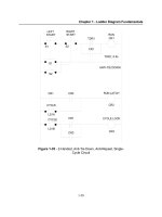
in Table 1.1.

Figure 1.6. (a) Foetal heart rate tracing with the vertical scale in b.p.m. (b) A detail
of the first prominent downward wave is shown with its primitives.

Table 1.1 Primitives of foetal heart rate tracings.
Primitive Name
Symbol
Description
h
A segment of constant value
Horizontal
u
An upward segment with slope < A
Up slope
Down slope
d
A downward segment with slope > - A
Strong up slope
U
An upward segment with slope 2 A

Strong down slope
D
A downward segment with slope I - A
A is a minimum slope value specified beforehand


I .2 Pattern Similarity and PR Tasks

9

Based on these elements we can describe a spike as any sequence consisting of a
subsequence of U primitives followed by a subsequence of D primitives or viceversa, with at least one U and one D and no other primitives between. Figures 1.7a
and 1.7b show examples of spikes and non-spikes according to this rule.

wave

n

II

other accel. decel.

n
wander shift

I

Figure 1.7 Wave primitives for FHR signal: (a) Spikes; (b) Non-spikes; (c) Wave
hierarchy.

The non-spikes could afterwards be classified as accelerations, decelerations or
other wave types. The rule for acceleration could be: any up wave sequence
starting with at least one u primitive with no d's in between, terminating with at
least one d primitive with no M'S inibetween. An example is shown at the bottom of
Figure 1.7b. With these rules we could therefore establish a hierarchy of wave
descriptions as shown in Figure 1 . 7 ~ .
In this description task the similarity of the objects (spikes, accelerations,
rule. Two
decelerations, etc., in this example) is assessed by means of a s~ruc~ural
objects are similar if they obey the same rule. Therefore all spikes are similar, all
accelerations are similar, and so on. Note in particular that the bottom spike of
Figure 1.7a is, in this sense, more similar to the top spike than the top wave of
Figure 1.7b, although applying a distance measure to the values of the signal
amplitudes, using the first peak as time alignment reference, would certainly lead
to a different result!
The structural rule is applied here to the encoded sequence of the primitives, in
the form of a string ofprimitives, in order to see if the rule applies. For instance, a
machine designed to describe foetal heart rate tracings would encode the segment
shown in Figure 1.6b as "uduDUuud",thereby recognizing the presence of a spike.

1.3 Classes, Patterns and Features
In the pattern recognition examples presented so far a quite straightforward
correspondence existed between patterns and classes. Often the situation is not that
simple. Let us consider a cardiologist intending to diagnose a heart condition based
on the interpretation of electrocardiographic signals (ECG). These are electric


10

1 Basic Notions

signals acquired by placing electrodes on the patient's chest. Figure 1.8 presents
four ECGs, each one corresponding to a distinct physiological condition:
N - normal; LVH - left ventricle hypertrophy; RVH - right ventricle hypertrophy;
MI - myocardial infarction.

Figure 1.8. ECGs of 4 diagnostic classes: (N) Normal; (LVH) Left ventricular
hypertrophy; (RVH) Right ventricular hypertrophy; (MI) Myocardial infarction.

Each ECG tracing exhibits a "wave packet" that repeats itself in a more or less
regular way over time. Figure 1.9 shows an example of such a "wave packet",
whose components are sequentially named P, Q, R, S and T. These waves reflect
the electrical activity of distinct parts of the heart. A P wave reflects the atrial
activity of the heart. The Q, R, S and T waves reflect the subsequent ventricular
activity.

Figure 1.9. ECG wave packet with sequentially named waveforms P, Q, R, S, T.

Cardiologists learn to interpret the morphology of these waves in
correspondence with the physiological state of the heart. The situation can be
summarized as follows:
-

-

There is a set of clusses (states) in whlch can be found a certain studied entity.
In the case of the heart we are considering the mentioned four classes.
Corresponding to each class (state) is a certain set of representations (signals,
images, etc.), thepatrerns. In the present case the ECGs are the patterns.

I .3 Classes, Patterns and Features

-

11

From each pattern we can extract information characterizing it, the features. In
the ECG case the features are related to wave measurements of amplitudes and
durations. A feature can be, for instance, the ratio between the amplitudes of the
Q and R waves, Q/R ratio.

In order to solve a PR problem we must have clear definitions of the class,
pattern and feature spaces. In the present case these spaces are represented in
Figure 1.10.

classes
(heart condition)

Patterns
(ECGs)

Features
(amplitudes, durations, ...)

Figure 1.10. PR spaces for the heart condition classification using ECG features.

A PR system emulating the cardiologist abilities, when presented with a feature
vector, would have to infer the heart condition (diagnostic class) from the feature
vector. The problem is that, as we see from Figure 1.10, there are annoying

overlaps: the same Q/R ratio can be obtained from ECGs corresponding to classes
N and LVH; the same ECG can be obtained from classes MI and RVH. The first
type of overlap can be remedied using additional features; the second type of
overlap is intrinsic to the method and, as a matter of fact, the best experts in
electrocardiography have an upper limit to their performance (about 23% overall
classification error when using the standard " 12-lead ECG system" composed of 12
ECG signals). Therefore, a PR system frequently has a non-zero performance error,
independent of whatever approach is used, and usually one is satisfied if it
compares equally or favourably with what human experts can achieve.
Sun~marizingsome notions:
Classes

Classes are states of "nature" or crrtegorirs of objects associated with concepts or
prototyyrs.
In what follows we assume c classes denoted (0, E Q , (i = 1,. . . .c ) , where R is
the set of all classes, known as the itllerpretutiotz spuce. The interpretation space
has cmcept-drivetz properties such as unions, intersections and hierarchical trees of
classes.