Springer stochastic linear programming models theory computation p kall j mayer (springer 2005) WW
Bạn đang xem bản rút gọn của tài liệu. Xem và tải ngay bản đầy đủ của tài liệu tại đây (16.6 MB, 405 trang )
STOCHASTIC LINEAR PROGRAMMING
Models, Theory, and Computation
PETER KALL
University of ZurichlSwitzerland
JANOS MAYER
University of ZurichlSwitzerland
Recent titles in the
INTERNATIONAL SERIES IN
OPERATIONS RESEARCH & MANAGEMENT SCIENCE
Frederick S. Hillier, Series Editor, Stanford
University
Zhul QUANTITATIVE MODELS FOR PERFORMANCE EVALUATION AND BENCHMARKING
Ehrgott & Gandibleux/MULTIPLE CRITERIA OPTIMIZATION: State of the Art Annotated
Bibliographical Surveys
Bienstockl Potential Function Methodsfor Approx. Solving Linear Programming Problems
Matsatsinis & Siskosl INTELLIGENTSUPPORTSYSTEMS FOR MARKETING
DECISIONS
Alpern & GaV THE THEORY OF SEARCH GAMES AND RENDEZVOUS
HalVHANDBOOK OF TRANSPORTATIONSCIENCE - 2" Ed.
Glover & Kochenberger/HANDBOOK OF METAHEURISTICS
Graves & RinguestJ MODELS AND METHODS FOR PROJECT SELECTION:
Conceptsfrom Management Science, Finance and Information Technology
Hassin & Havivl TO QUEUE OR NOT TO QUEUE: Equilibrium Behavior in Queueing Systems
Gershwin et avANALYSIS & MODELING OF MANUFACTURING SYSTEMS
Marosl COMPUTATIONAL TECHNIQUES OF THE SIMPLEX METHOD
Harrison, b e & Nealel THE PRACTICE OF SUPPLY CHAIN MANAGEMENT: Where Theory and
Application Converge
Shanthikumar, Y a o & Zijml STOCHASTIC MODELING AND OPTIMIZATION OF
MANUFACTURING SYSTEMS AND SUPPLY CHAINS
l
RESOURCE MANAGEMENT: State of the Art and Future
Nabrzyski, Schopf & W ~ g l a r zGRID
Trends
Thissen & Herder1 CRITICAL INFRASTRUCTURES: State of the Art in Research and Application
Carlsson, Fedrizzi, & FullBrl FUZZY LOGIC IN MANAGEMENT
Soyer, Mazzuchi & Singpurwalld MATHEMATICAL RELIABILITY: An Expository Perspective
Chakravarty & Eliashbergl MANAGING BUSINESS INTERFACES: Marketing, Engineering, and
Manufacturing Perspectives
Talluri & van Ryzinl THE THEORYAND PRACTICE OF REVENUE MANAGEMENT
Kavadias & LochlPROJECT SELECTION UNDER UNCERTAINTY: Dynamically Allocating
Resources to Maximize Value
Brandeau, Sainfort & Pierskallal OPERATIONS RESEARCHAND HEALTH CARE:A Handbookof
Methods and Applications
Cooper, Seiford & Zhul HANDBOOK OF DATA ENVELOPMENTANALYSIS: Models and Methods
Luenbergerl LINEAR AND NONLINEAR PROGRAMMING, 2" Ed.
Sherbrookel OPTIMAL INVENTORY MODELING OF SYSTEMS: Multi-Echelon Techniques,
Second Edition
Chu, Leung, Hui & Cheungl4th PARTY CYBER LOGISTICS FOR AIR CARGO
S i m c h i - b v i , Wu & S h e d HANDBOOK OF QUANTITATIVE SUPPLY CHAIN ANALYSIS:
Modeling in the E-Business Era
Gass & Assadl AN ANNOTATED TIMELINE OF OPERATIONS RESEARCH: An Informal History
Greenberg/ TUTORIALS ON EMERGING METHODOLOGIES AND APPLICATIONS IN
OPERATIONS RESEARCH
Weberl UNCERTAINTYIN THE ELECTRIC POWER INDUSTRY: Methods and Modelsfor Decision
Support
Figueira, Greco & EhrgottJ MULTIPLE CRITERIA DECISIONANALYSIS: State of the Art Surveys
Reveliotisl REAL-TIME MANAGEMENT OF RESOURCE ALLOCATIONS SYSTEMS: A Discrete
Event Systems Approach
* A list of the early publications in the series is at the end of the book *
STOCHASTIC LINEAR PROGRAMMING
Models, Theory, and Computation
PETER KALL
University of ZurichlSwitzerland
JANOS MAYER
University of ZurichlSwitzerland
Q
- Springer
Peter Kall
University of Zurich
Switzerland
JAnos Mayer
University of Zurich
Switzerland
Library of Congress Cataloging-in-Publication Data
A C.I.P. Catalogue record for this book is available
from the Library of Congress.
ISBN 0-387-23385-7
e-ISBN 0-387-24440-9
Printed on acid-free paper.
Copyright O 2005 by Kluwer Academic Publishers.
All rights reserved. This work may not be translated or copied in whole or in
part without the written permission of the publisher (Springer Science +
Business Media, Inc., 233 Spring Street, New York, NY 10013, USA), except
for brief excerpts in connection with reviews or scholarly analysis. Use in
connection with any form of information storage and retrieval, electronic
adaptation, computer software, or by similar or dissimilar methodology now
know or hereafter developed is forbidden.
The use in this publication of trade names, trademarks, service marks and
similar terms, even if the are not identified as such, is not to be taken as an
expression of opinion as to whether or not they are subject to proprietary rights.
Printed in the United States of America.
9 8 7 6 5 4 3 2 1
SPIN 11050001
Contents
Notations
Preface
1. BASICS
1
Introduction
2
Linear Programming Prerequisites
2.1
Algebraic concepts and properties
2.2
Geometric interpretation
2.3
Duality statements
2.4
The Simplex Method
2.5
The Dual Simplex Method
2.6
Dual Decomposition
2.7
Nested Decomposition
2.8
Regularized Decomposition
2.9
Interior Point Methods
3
Nonlinear Programming Prerequisites
3.1
Optimality Conditions
3.2
Solution methods
2. SINGLE-STAGE SLP MODELS
1
Introduction
2
Models involving probability functions
2.1
Basic properties
2.2
Finite discrete distribution
2.3
Separate probability functions
2.3.1 Only the right-hand-side is stochastic
2.3.2 Multivariate normal distribution
STOCHASTIC LINEAR PROGRAMMING
3
4
5
6
7
Stable distributions
A distribution-free approach
The independent case
Joint constraints: random right-hand-side
Generalized-concave probability measures
Generalized-concave distribution functions
Maximizing joint probability functions
Joint constraints: random technology matrix
Summary on the convex programming subclasses
Quantile functions, Value at Risk
Models based on expectation
4.1
Integrated chance constraints
4.1.1 Separate integrated probability functions
4.1.2 Joint integrated probability functions
4.2
A model involving conditional expectation
4.3
Conditional Value at Risk
Models built with deviation measures
5.1
Quadratic deviation
5.2
Absolute deviation
5.3
Quadratic semi-deviation
5.4
Absolute semi-deviation
Modeling risk and opportunity
Risk measures
7.1
Risk measures in finance
7.2
Properties of risk measures
7.3
Portfolio optimization models
3. MULTI-STAGE SLP MODELS
The general SLP with recourse
1
2
The two-stage SLP
2.1
Complete fixed recourse
2.2
Simple recourse
Some characteristic values for two-stage SLP's
2.3
3
The multi-stage SLP
3.1
MSLP with finite discrete distributions
3.2
MSLP with non-discrete distributions
4. ALGORITHMS
1
Introduction
vii
2
3
4
5
6
7
Single-stage models with separate probability functions
2.1
A guide to available software
Single-stage models with joint probability functions
3.1
Numerical considerations
3.2
Cutting plane methods
3.3
Other algorithms
3.4
Bounds for the probability distribution function
3.5
Computing probability distribution functions
3.5.1 A Monte-Carlo approach with antithetic variates
3.5.2 A Monte-Carlo approach based on probability bounds
3.6
Finite discrete distributions
A guide to available software
3.7
3.7.1 SLP problems with logconcave distribution functions
3.7.2 Evaluating probability distribution functions
3.7.3 SLP problems with finite discrete distributions
Single-stage models based on expectation
4.1
Solving equivalent LP's
4.2
Dual decomposition revisited
4.3
Models with separate integrated probability functions
4.4
Models involving CVaR-optimization
4.5
Models with joint integrated probability functions
A guide to available software
4.6
4.6.1 Models with separate integrated probability functions
4.6.2 Models with joint integrated probability functions
4.6.3 Models involving CVaR
Single-stage models involving VaR
Single-stage models with deviation measures
A guide to available software
6.1
Two-stage recourse models
7.1
Decomposition methods
7.2
Successive discrete approximation methods
7.2.1 Computing the Jensen lower bound
7.2.2 Computing the E-M upper bound for an interval
7.2.3 Computing the bounds for a partition
7.2.4 The successive discrete approximation method
7.2.5 Implementation
7.2.6 Simple recourse
7.2.7 Other successive discrete approximation algorithms
viii
STOCHASTIC LINEAR PROGRAMMING
7.3
Stochastic algorithms
7.3.1 Sample average approximation (SAA)
7.3.2 Stochastic decomposition
7.3.3 Other stochastic algorithms
7.4
Simple recourse models
7.5
A guide to available software
8
Multistage recourse models
8.1
Finite discrete distribution
8.2
Scenario generation
8.2.1 Bundle-based sampling
8.2.2 A moment-matching heuristic
8.3
A guide to available software
9
Modeling systems for SLP
Modeling systems for SLP
9.1
SLP-IOR
9.2
9.2.1 General issues
9.2.2 Analyze tools and workbench facilities
9.2.3 Transformations
9.2.4 Scenario generation
9.2.5 The solver interface
9.2.6 System requirements and availability
References
Index
342
342
348
352
353
353
356
356
358
360
361
367
368
368
369
370
371
372
372
373
374
375
395
Notations
One-stage models: Joint chance constraints
arrays (usually given real matrices)
arrays (usually given real vectors)
arrays (usually real or integer variable vectors)
probability space
set of natural numbers
IRT endowed with the Borel a-algebra BT
random vector, i.e. Borel measurable mapping
inducing the probability measure IPt on BT
according to IPt(M) = P(t-l[M]) VM E BT
random array and random vector, respectively,
defined as:
h(t) = h
+
h j t j ; h, h j E IRm2 fix
j=1
expectation
expectations IE+[T(J)] = ~ ( f and
)
lE+ [h(t)] = h(f), respectively
realization of random t
realizations ~ ( 8 h,( 6 , respectively
One-stage models: Separate chance constraints
:
i-th row of T(.)
:
i-th component of h(-)
Two-stage recourse models
:
random array and random vector, respectively,
defined as:
x
STOCHASTIC LINEAR PROGRAMMING
T
W ( . ) : l R r + l R m 2 x n 2:
W ( J ) = W + ~ W ~ & ;wW ~,
E
I
R
~
~
j=1
r
q(.) : lRr + lRn2
:
q(~)=q+C$~j;q7qi~~n2
j=1
-
w,
:
(c)and
expectations IE+ [W( J ) ] = W
JEc [4(5)]= q(C),respectively
Multi-stage recourse models
J:fl+lRR
:
random vector J = ( J 2 , . . . ,J T )with
T
J t : n + I R r t ,t = 2 , . . . , T a n d x r t = R
t=2
Ct
: f l + lRRt
:
the state of the process at stage t, defined as
random vector St = ( J 2 , - . . ,J t ) , t 1 2, or else
t
St
= (ql,.. . ,
with Rt =
C r,, with the
~ = 2
corresponding marginal distribution of J
n=2 U=R,-~+I
where At,, At,, E lRmtXnr
and R1 = 0,
withl<~
Multi-stage recourse models: Discrete distribution
J:n+lRR
:
random vector with discrete distribution
qs);s = 1, ,S ) , @.
scenarios J = (Jl,
- . ,J;) = . . . ,T i )
with IPE(J = J S ) = qs, s E S := (1, -.. ,S )
{(p,
A
(e.,
A
A
Ct : f2 + lRRt
A
:
discrete set {C,S =
(e,. . . ,@); s E S ) of
A
~
states defining kt 2 1 different equivalence
=
classes U,V S, with s i , sj E U,V H
and an associated set of different states at
stage t which may be defined by
St := { p I p minimal in one of the U,V)
as
I p E St) with the distribution
ci
(2
=v)=
PI(G
n
Ttp
I
=
sES
e -ct I
s
- ^P
(see Fig. 1 with e.g. Sz = {1,6,11))
Figure 1. Scenario tree: Assigning states to nodes.
xii
STOCHASTIC LINEAR PROGRAMMING
Multi-staee recourse models: The scenario tree
(N,4
tree with nodes N c IN,where n = 1 is the
T
+
(unique) root and I NI =
I StI 1
t=2
the stage to which n E N belongs;
there is a bijection
tn
w- {lH
@I.},~ ( 9 :)
T
U{(t,~t)}
t=2
such that n tt (tn, p(n)), n 2 2;
hence we assign with any node n 2 2
p
P
D(t)
c(n){zP!"),
=
with
p(n) E St,} uniquely
determined by n E N (state in node n)
cN
set of nodes in stage t, 1 5 t 5 T
the parent node of node n E N, n 2 2
(immediate predecessor)
hn
B(n)
+
cN
set of nodes in the path from n E N to the root,
ordered by stages, including n (history of n)
2 p},
S(n) = {s E S I
=
i.e. the index set
of those scenarios, for which the scenario path
contains n E N. S ( n ) and the related set of
scenarios are called the scenario bundle of
the corresponding node n
set of children (immediate successors) of n
future of node n along scenario s E S(n),
including n (and hence Gs(n) = 0 if s 6B(n))
To Helene and Ilona
Preface
The beginning of stochasticprogramming, and in particular stochastic linear
programming (SLP), dates back to the 50's and early 60's of the last century.
Pioneers w h e a t that time-contributed to the field, either by identifying SLP
problems in particular applications, or by formulating various model types and
solution approaches for dealing adequately with linear programs containing
random variables in their right-hand-side, their technology matrix, andlor their
objective's gradient, have been among others (in alphabetical order):
E.M.L. Beale [lo], proposing a quadratic programming approach to solve special simple recourse stochastic programs;
A. Charnes and W.W. Cooper [38], introducing a particular stochastic program
with chance constraints;
G.B. Dantzig [43], formulating the general problem of linear programming with
uncertain data and
G.B. Dantzig and A. Madansky [47], discussing at an early stage the possibility
to solve particular two-stage stochastic linear programs;
G. Tintner [287], considering stochastic linear programming as an appropriate
approach to model particular agricultural applications; and
C. van de Panne and W. Popp [293], considering a cattle feed problem modeled
with probabilistic constraints.
In addition we should mention just a few results and methods achieved before
1963, which were not developed in connection with stochastic programming,
but nevertheless turned out to play an essential role in various areas of our field.
One instance is the Brunn-Minkowski inequality based on the investigations
of H. Brunn [32] in 1887 and H. Minkowski [206] in 1897, which comes
up in connection with convexity statements for probabilistic constraints, as
mentioned e.g. in Prkkopa [234]. Furthermore, this applies in particular to
the discussion about bounds on distribution functions, based on inequalities
published by G. Boole in 1854and by C.E. Bonferroni in 1937 (for the references
4
STOCHASTIC LINEAR PROGRAMMING
see Prkkopa [234]), and on the other hand, about bounds on the expectation of a
convex function of a random variable, leading to a lower bound by the inequality
of J.L. Jensen [128], and to the Edmundson-Madansky upper bound due to
H.P. Edmundson [7 11 and A. Madansky [1831.
Among the concepts of solution approaches, developed until 1963 for linear
or nonlinear programming problems, the following ones, in part after appropriate modifications, still serve as basic tools for dealing with SLP problems:
Besides Dantzig's simplex method and the Dantzig-Wolfe decomposition, described in detail in G.B. Dantzig [44], the dual decomposition proposed by
J.F. Benders [12], cutting plane methods as introduced by J.E. Kelley [159],
and feasible direction methods proposed and discussed in detail by G. Zoutendijk [311], may be recognized even within today's solution methods for
various SLP problems. Of course, these methods and in particular their implementations have been revised and improved meanwhile, and in addition we
know of many new solution approaches, some of which will be dealt with in
this book.
The aim of this volume is to draw a bow from solution methods of (deterministic) mathematical programming, being of use in SLP as well, through
theoretical properties of various SLP problems which suggest in many cases the
design of particular solution approaches,to solvers, understood as implemented
algorithms for the solution of the corresponding SLP problems.
Obviously we are far from giving a complete picture on the present knowledge and computational possibilities in SLP. First we had to omit the area
of stochastic integer programming (SILP), since following the above concept
would have implied to give first a survey on those integer programming methods used in SILP; this would go beyond the limits of this volume. However
the reader may get a first flavour of SILP by having a look for instance into
the articles of W.K. Klein Haneveld, L. Stougie, and M.H. van der Vlerk [168],
W. Romisch and R. Schultz [256], M.H. van der Vlerk [299], and the recent
survey of S. Sen [268].
And, as the second restriction, in presenting detailed descriptions we have
essentially confined ourselves to those computational methods for solving SLP
problems belonging to one of the following categories:
Either information on the numerical efficiency of a corresponding solver is
reported in the literature based on reasonable test sets (not just three examples
or less!) and the solver is publicly available;
or else, corresponding solvers have been attached to our model management
system SLP-IOR, either implemented by ourselves or else provided by their
authors, such that we were able to gain computationalexperienceon the methods
presented, based on running the corresponding solvers on randomly generated
test batteries of SLP's with various characteristics like problem size, matrix
PREFACE
5
entries density, probability distribution, range and sign of problem data, and
some others.
Finally, we owe thanks to many colleagues for either providing us with
their solvers to link them to SLP-IOR, or for their support in implementing
their methods by ourselves. Further, we gratefully acknowledge the critical
comments of Simon Siegrist at our Institute. Obviously, the remaining errors
are the sole responsibility of the authors. Last but not least we are indebted
to the publisher for an excellent cooperation. This applies in particular to the
publisher's representative, Gary Folven, to whom we are also greatly obliged
for his patience.
Ziirich, September 2004
Peter Kall and J h o s Mayer
Chapter 1
BASICS
1.
Introduction
Linear programs have been studied in many aspects during the last 50 years.
They have shown to be appropriate models for a wide variety of practical problems and, at the same time, they became numerically tractable even for very
large scale instances. As standard formulations of linear programs (LP) we find
problems like
subject to
min cTx
Ax cc b
l
<
}
(1.1)
with the matrix A E IRmXn,the objective's gradient c E IRn, the righthand-side b E IRm, and the lower and upper bounds 1 E IRn and u E lRn,
respectively. If some xi is unbounded below andor above, this corresponds to
li = -w andor ui = w. A,b, C,I, u are assumed to be known fixed data in
the above model. The relation 'cc' is to be replaced row-wise by one of the
relations '5' , '=' ,or '2' . Then the task is obviously to find the-or at least
one-optimal feasible solution x E lRn. Alternatively, we often find also the
LP-formulation
min cTx
subject to Ax cc b
1. 0,
(1.2)
under the analogous assumptions as above. For these two LP types it holds
obviously that, given a problem of one type, it may be reformulated into an
equivalent problem of the other type. More precisely,
8
STOCHASTIC LINEAR PROGRAMMING
given the LP in the formulation (1.2), by introducing the lower bounds
1 = (0, . . . ,o ) and
~ the upper bounds u = (co,. . . ,oo)* (in computations rather markers u = (M, . . ,M ) with
~ a sufficiently large number
M , e.g. M = lo2', just to indicate unboundedness), the problem is trivially of the type (1.1); and
having the LP of type (1.1), introducing variables x+ E IR?, x- E
IR?, inserting x = x+ - x-, x+ 2 0, x- 2 0, introducing the slack
variables y E IRn+and t E IR?, and restating the conditions 1 < x < u
equivalently as
the problem is transformed into the type (1.2).
In the same way it follows that every LP may be written as
min cTx
subject to Ax = b
x 2 0,
i.e. as a special variant of (1.2).
Numerical methods known to be efficient in solving LP's belong essentially
to one of the following classes:
- Pivoting methods, in particular the simplex andlor the dual simplex
method;
- interior point methods for LP's with very sparse matrices;
- decomposition, dual decomposition and regularized decomposition approaches for LP's with special block structures of their coefficient matrices A.
In real life problems the fimdamental assumption for linear programming,
that the problem entries--except for the variables x-be known fixed data, does
often happen not to hold. It either may be the case that (some of) the entries
are constructed as statistical estimates from some observed real data, i.e. from
some samples, or else that we know from the model design that they are random
variables (like capacities, demands, productivities or prices). The standard approach to replace these random variables by their mean values-corresponding
to the choice of statistical estimates mentioned before-and afterwards to solve
the resulting LP may be justified only under special conditions; in general, it
can easily be demonstrated to be dramatically wrong.
Basics
Assume, for instance, as a model for a diet problem the LP
min cTx
s. t. Ax 2: b
x 2: 0,
where x represents the quantities of various foodstuffs, and c is the corresponding price vector. The constraints reflect chemical or physiological requirements
to be satisfied by the diet. Let us assume that the elements of A and b are fixed
known data, i.e. deterministic,whereas at least some ofthe elements o f T andlor
h are random with a known joint probability distribution, which is not influenced by the choice of the decision x. Further, assume that the realizations of
the random variables in T and h are not known before the decision on the diet
x is taken, i.e. before the consumption of the diet. Replacing the random T and
h by their expectations T and and solving the resulting LP
z
min cTx
s.t. Ax 2: b
x 2: 0,
can result in a diet P violating the constraints in (1.4) very likely and hence
with a probability much higher than feasible for the diet to serve successfully
its medical purpose. Therefore, the medical experts would rather require a
decision on the diet which satisfies all constraints jointly with a rather high
probability, as 95% say, such that the problem to solve were
min cTx
s. t.
Ax 2: b
P ( T x 2: h) 2 0.95
x 2: 0,
a stochastic linearprogram (SLP) withjointprobabilistic constraints. Here we
had at the starting point the LP (1.4) as model for our diet problem. However,
the (practical) requirement to satisfy--besides the deierministic constraints
Ax 2 b-also the reliability constraint P ( T x 2: h) 2: 0.95, yields with (1.6) a
nonlinear program (NLP). This is due to the fact, that in general the probability
function G ( x ) := P ( T x 2: h) is clearly nonlinear.
As another example, let some production problem be formulated as
STOCHASTIC LINEAR PROGRAMMING
min cTx
s.t. Ax = b
Tx = h
x 2 0,
where T and h may contain random variables (productivities, demands, capacities, etc.) with a joint probability distribution (independent again of the
choice of x), and the decision on x has to be taken before the realization of
the random variables is known. Consequently, the decision x will satisfy the
constraints Ax = b, x > 0; but after the observation of the random variables'
realization it may turn out that T x # h, i.e. that part of the target (like satisfying
the demand for some of the products, capacity constraints, etc.) is not properly met. However, it may be necessary-by a legal commitment, the strong
intention to maintain goodwill, or similar reasons-to compensate for the deficiency, i.e. for h - Tx, after its observation. One possibility to cope with
this obligation may be the introduction of recourse by defining the constraints
Wy = h - Tx, y 2 0, for instance as model of an emergency production
process or simply as the measurement of the absolute values of the deficiencies
(represented by W = ( I , -I), with I the identity matrix). Let us assume W to
be deterministic, and assume the recourse costs to be given as linear by qTy, say.
Obviously we want to achieve this compensation with minimal costs. Hence
we have the recourse problem
For any x, feasible to thejrst stage constraints Ax = b, x 2 0, the recourse
function, i.e. the optimal value Q(x; T, h) of the second stage problem (1.8),
depends on T and h and is therefore a random variable. In many applications,
e.g. in cases where the production plan x has to be implemented periodically
(daily or weekly, for instance), it may be meaningkl to choose x in such a
way that the average overall costs, i.e. the sum of the first stage costs cTx and
the expected recourse costs IE Q(x; T, h), are minimized. Hence we have the
problem
+
min cTx IE Q(x; T, h)
s.t. Ax = b
x L 0,
(1.9)
a two-stage stochastic linear program (SLP) with Jixed recourse.
Also in this case, although our starting point was the LP (1.7), the resulting problem (1.9) will be an NLP if the random variables in T and h have a
11
Basics
continuous-typejoint distribution (i.e. a distribution defined by a density function).
If, however, the random variables in T and h have a joint discrete distribution,
defined by the realizations ( ~ jhj)
, with the pr~babilitiesp~,
j = 1,- . . ,S (with
S
pj
> 0 and
pj = I), problem (1.9) is easily seen to be equivalent to
j=l
S
rnin cTx
+ CpjpTyj
j=l
s. t.
Ax
= b
+Wyj = hj, j = l , . . . , S
2 0
x
Yj - 0,
T ~ X
.
1
(1.10)
such that under the discrete distribution assumption we get an LP again, with
the special data structure indicated in Fig. 1.1.
Figure 1.1. Dual decomposition structure.
In applications we observe an increasing need to deal with a generalization
of the two-stage SLP with recourse (1.9) and (1. lo), respectively. At this point
we just give a short description as follows: In a first stage, a decision x l is
chosen to be feasible with respect to some deterministic first stage constraints.
Later on, after the realization of a random vector (2, a deficiency in some
second stage constraints has to be compensated for by ah appropriate recourse
the
decision x2(J2). Then after the realization of a further random vector 6,
former decisions x1 and x2 (&) may not be feasible with respect to some third
stage constraints, and a further recourse decision x3(t2,53) is needed, and so
on, until a final stage T is reached. Again, we assume that, besides the first
stage costs cTxl, the recourse decisions xt(Ct), t 1. 2, imply additional linear
12
STOCHASTIC LINEAR PROGRAMMING
costs cTxt ( ~ t )where
,
Ct = (E2,
recourse is formulated as
+
. ,&).
Then the multi-stage SLP with f i e d
subject to
where, in general, we shall assume Att(Ct), t 2 2, the matrices on the diagonal, to be deterministic, i.e. Att(Ct) Att. It will turn out that, for general
probability distributions, this problem-an NLP again-is much more difficult
than the two-stage SLP (1.9), and methods to approximate a solution are just
at their beginning phase, at best. However, under the assumption of discrete
distributions of the random vectors Ct, problem (1.1 1) can also be reformulated
into an equivalent LP, which in general is of (very) large scale, but again with
a special data structure to be of use for solution procedures.
From this short sketch of the subject called SLP, which is by far not complete
with respect to the various special problem formulations to be dealt with, we
may already conclude that a basic toolkit of linear and nonlinear programming
methods cannot be waived if we want to deal with the computational solution
of SLP problems. To secure the availability of these resources, in the following
sections of this chapter we shall remind to basic properties of and solution
methods for LP's and NLP's as they are used or referred to in the SLP context,
later on.
In Chapter 2, we present various Single-stage SLP models (like e.g. problem (1.6) on page 9) and discuss their theoretical properties, relevant for their
computational tractability, as convexity statements, for instance.
In Chapter 3 follows an anlogous discussion of Multi-stage SLP models (like
problem (1.9) in particular, and problem (1.11) in genekal), focussed among
others on properties allowing for the construction of particular approximation
methods for computing (approximate) solutions.
For some of the models discussed before, Chapter 4 will present solution
methods, which have shown to be efficient in extensive computational experiments.
13
Basics
Linear Programming Prerequisites
2.
In this section we briefly present the basic concepts in linear programming
and, for various types of solution methods, the conceptual algorithms.
As mentioned on page 8 we may use the following standard formulation of
an LP:
min cTx
s.t. Ax = b
x 2 0.
1
With A being an ( m x n)-matrix, and b and c having correspondingdimensions,
we know from linear algebra that the system of equations
Ax = b is solvable if and only if rank(A, b) = rank(A).
Therefore, solvability of the system Ax = b implies that
either rank(A) = m,
or the system contains redundant equations which may be omitted, such that
for the remaining system Ax = 6 we have the same set of solutions as for
the original system, and that, for the (ml x n)-matrix A, m l < m, the
condition rank(A) = m l holds.
Observing this well known fact, we henceforth assume without loss of generality, that rank(A) = m ( 5 n) for the (m x n)-matrix A.
2.1
Algebraic concepts and properties
Solving the LP (2.1) obviously requires to find an extreme (minimal in our
formulation) value of a linear function on a feasible set described as the intersection of a linear manifold, {x I Ax = b } , and finitely many halfspaces,
{x I x j :j 01, j = 1,. - ,n, suggesting that this problem may be discussed in
algebraic terms.
DEFINITION2.1 Any feasible solution P of (2.1) is called a feasible basic
solution if; for I(?) = { i 1 2 > O}, the set {Ai, i E I(P)) of columns in A is
linearly independent.
According to this definition, for any feasible basic solution P of (2.1) holds
Pi > O f o r i E I(?),
1-, = O f o r j @ I(*),
Ai&= b.
and
iEZ(&)
Furthermore, with I I(2) I being the cardinality of this set (i.e. the number of
its elements), if II(P)l < m such that the basic solution P contains less than
14
STOCHASTIC LINEAR PROGRAMMING
m strictly positive components, then due to our rank assumption on A there
is a subset IB(2) with IB(2) > I ( 2 ) and IIB(2) I = m such that the column set {Ai,i E IB(2)} is linearly independent or equivalently, that the
(m x m)-matrix B = (Ai I i E IB(2)) is nonsingular. Introducing, with
} IN(*) = { I l . . - , n } \ IB(2) = { j l l - ~ ~ , j n - m } ,
IB(2) = { i l , - + + , i mand
the vectors xtB) E Rm-the basic variables-and x { ~ )E Rn-m-the nonbasic variables-according to
then, with the (m x (n-m))-matrix N = (Aj I j E IN( 2 ) )the system Ax = b
is, up to a possible rearrangement of columns and variables, equivalent to the
system
BxtB) N X { ~ ) = b.
+
Therefore, up to the mentioned rearrangement of variables, the former feasible
basic solution 2 corresponds to (2tB) = B-lb 2 0, ktN) = O), and the
submatrix B of A is called a feasible basis . With the same rearrangement of
the components of the vector c into the two vectors ctB) and ctN) we may
rewrite problem (2.1) as
Solving the system of equations for xiB) we get xtB) = B-lb - B d l ~ x t N )
T
such that-with y~ := ctB) B-lb the objective value of the feasible basic
solution (piB) = B-lb 2 0, 2{N) = 0)-problem (2.1) is equivalent to
For computational purposes (2.2) is usually represented by the simplex tableau
Qmn-m
such that the objective and the equality constraints of (2.2) are rewritten as