Advanced analysis and learning on temporal data first ECML PKDD workshop, AALTD 2015

LNAI 9785

Ahlame Douzal-Chouakria · José A. Vilar
Pierre-François Marteau (Eds.)

Advanced Analysis
and Learning
on Temporal Data
First ECML PKDD Workshop, AALTD 2015
Porto, Portugal, September 11, 2015
Revised Selected Papers

123


Lecture Notes in Artificial Intelligence
Subseries of Lecture Notes in Computer Science

LNAI Series Editors
Randy Goebel
University of Alberta, Edmonton, Canada
Yuzuru Tanaka
Hokkaido University, Sapporo, Japan
Wolfgang Wahlster
DFKI and Saarland University, Saarbrücken, Germany

LNAI Founding Series Editor
Joerg Siekmann
DFKI and Saarland University, Saarbrücken, Germany

9785

More information about this series at />

Ahlame Douzal-Chouakria José A. Vilar
Pierre-François Marteau (Eds.)
•

Advanced Analysis
and Learning
on Temporal Data
First ECML PKDD Workshop, AALTD 2015
Porto, Portugal, September 11, 2015
Revised Selected Papers

123


Editors
Ahlame Douzal-Chouakria
Laboratoire d’Informatique de Grenoble
Université Grenoble Alpes (UGA)
Grenoble
France

Pierre-François Marteau
IRISA
Université de Bretagne-Sud
Vannes
France

José A. Vilar
Universidade da Coruna
Coruna
Spain

ISSN 0302-9743
ISSN 1611-3349 (electronic)
Lecture Notes in Artificial Intelligence
ISBN 978-3-319-44411-6
ISBN 978-3-319-44412-3 (eBook)
DOI 10.1007/978-3-319-44412-3
Library of Congress Control Number: 2016947506
LNCS Sublibrary: SL7 – Artificial Intelligence
© Springer International Publishing Switzerland 2016
This work is subject to copyright. All rights are reserved by the Publisher, whether the whole or part of the
material is concerned, specifically the rights of translation, reprinting, reuse of illustrations, recitation,
broadcasting, reproduction on microfilms or in any other physical way, and transmission or information
storage and retrieval, electronic adaptation, computer software, or by similar or dissimilar methodology now
known or hereafter developed.
The use of general descriptive names, registered names, trademarks, service marks, etc. in this publication
does not imply, even in the absence of a specific statement, that such names are exempt from the relevant
protective laws and regulations and therefore free for general use.
The publisher, the authors and the editors are safe to assume that the advice and information in this book are
believed to be true and accurate at the date of publication. Neither the publisher nor the authors or the editors
give a warranty, express or implied, with respect to the material contained herein or for any errors or
omissions that may have been made.
Printed on acid-free paper
This Springer imprint is published by Springer Nature
The registered company is Springer International Publishing AG Switzerland

Preface

This book brings together advances and new perspectives in machine learning,
statistics, and data analysis on temporal data. Temporal data arise in several domains
such as bio-informatics, medicine, finance, and engineering, among many others. They
are naturally present in applications covering language, motion, and vision analysis,
and particularly in emerging applications such as energy-efficient building, smart cities,
dynamic social media, or Internet of Things. Contrary to static data, temporal data are
of a complex nature, they are generally noisy, of high dimensionality, they may be
nonstationary (i.e., first-order statistics vary with time) and irregular (involving several
time granularities), they may have several invariant domain-dependent factors such as
time delay, translation, scale, or tendency effects. These temporal peculiarities make
limited the majority of standard statistical models and machine learning approaches,
that mainly assume i.i.d. data, homoscedasticity, normality of residuals, etc. To tackle
such challenging temporal data, one appeals for new advanced approaches at the bridge
of statistics, time series analysis, signal processing, and machine learning. Defining
new approaches that transcend boundaries between several domains to extract valuable
information from temporal data will undeniably be a hot topic in the near future, that
has, however, been the subject of active research this past decade.
The aim of this book is to present recent challenging issues and advances in temporal data analysis addressed in machine learning, data mining, pattern analysis and
statistics. Analysis and learning from temporal data cover a wide scope of tasks
including learning metrics, learning representations, unsupervised feature extraction,
clustering, and classification. This book is organized as follows. The first part focuses
on learning new representations and embeddings for time series classification, clustering, or dimensionality reduction. The second chapter presents several approaches to
classification and clustering with challenging applications in medicine or earth observation data. These works show different ways to consider temporal dependency in
clustering or classification processes. The last part of the book is dedicated to metric
learning and time series comparison, it addresses the problem of speeding up the
dynamic time warping or dealing with multimodal and multiscale metric learning for

time series classification and clustering. The papers presented were reviewed by at least
two independent reviewers, leading to the selection of 11 papers among 22 initial
submissions. An index of authors is provided at the end of this book.
The editors are grateful to the authors of the papers selected in this volume for their
contributions and for their willingness to respond so positively to the time constraints in
preparing the final version of their papers. We are especially grateful to the reviewers,
listed herein, for their careful reviews that helped us greatly in selecting the papers


VI

Preface

included in this volume. We also thank all the staff at Springer for their support and
dedication in publishing this volume in the series–Lecture Notes in Artificial
Intelligence.
July 2015

Ahlame Douzal-Chouakria
José A. Vilar
Pierre-François Marteau
Ann E. Maharaj
Andrés M. Alonso
Edoardo Otranto
Irina Nicolae


Organization

Program Committee

Ahlame Douzal-Chouakria
José Antonio Vilar Fernández
Pierre-François Marteau
Ann Maharaj
Andrés M. Alonso
Edoardo Otranto

Université Grenoble Alpes, France
University of A Coruña, Spain
IRISA, Université de Bretagne-Sud, France
Monash University, Australia
Universidad Carlos III de Madrid, Spain
University of Messina, Italy

Reviewing Committee
Massih-Reza Amini
Manuele Bicego
Gianluca Bontempi
Antoine Cornuéjols
Pierpaolo D’Urso
Patrick Gallinari
Eric Gaussier
Christian Hennig
Frank Höeppner
Paul Honeine
Vincent Lemaire
Manuel García Magariños
Mohamed Nadif
François Petitjean
Fabrice Rossi

Allan Tucker

Université Grenoble Alpes, France
University of Verona, Italy
MLG, ULB University, Belgium
LRI, AgroParisTech, France
La Sapienza University, Italy
LIP6, Université Pierre et Marie Curie, France
Université Grenoble Alpes, France
London’s Global University, UK
Ostfalia University of Applied Sciences, Germany
ICD, Université de Troyes, France
Orange Lab, France
University of A Coruña, Spain
LIPADE, Université Paris Descartes, France
Monash University, Australia
SAMM, Université Paris 1, France
Brunel University, UK


Contents

Time Series Representation and Compression
Symbolic Representation of Time Series: A Hierarchical Coclustering
Formalization . . . . . . . . . . . . . . . . . . . . . . . . . . . . . . . . . . . . . . . . . . . . .
Alexis Bondu, Marc Boullé, and Antoine Cornuéjols

3

Dense Bag-of-Temporal-SIFT-Words for Time Series Classification . . . . . . .

Adeline Bailly, Simon Malinowski, Romain Tavenard, Laetitia Chapel,
and Thomas Guyet

17

Dimension Reduction in Dissimilarity Spaces for Time Series Classification . . .
Brijnesh Jain and Stephan Spiegel

31

Time Series Classification and Clustering
Fuzzy Clustering of Series Using Quantile Autocovariances . . . . . . . . . . . . .
Borja Lafuente-Rego and Jose A. Vilar

49

A Reservoir Computing Approach for Balance Assessment . . . . . . . . . . . . .
Claudio Gallicchio, Alessio Micheli, Luca Pedrelli, Luigi Fortunati,
Federico Vozzi, and Oberdan Parodi

65

Learning Structures in Earth Observation Data with Gaussian Processes. . . . .
Fernando Mateo, Jordi Muñoz-Marí, Valero Laparra, Jochem Verrelst,
and Gustau Camps-Valls

78

Monitoring Short Term Changes of Infectious Diseases in Uganda
with Gaussian Processes. . . . . . . . . . . . . . . . . . . . . . . . . . . . . . . . . . . . . .

Ricardo Andrade-Pacheco, Martin Mubangizi, John Quinn,
and Neil Lawrence
Estimating Dynamic Graphical Models from Multivariate Time-Series
Data: Recent Methods and Results . . . . . . . . . . . . . . . . . . . . . . . . . . . . . .
Alex J. Gibberd and James D.B. Nelson

95

111

Metric Learning for Time Series Comparison
A Multi-modal Metric Learning Framework for Time Series
kNN Classification . . . . . . . . . . . . . . . . . . . . . . . . . . . . . . . . . . . . . . . . .
Cao-Tri Do, Ahlame Douzal-Chouakria, Sylvain Marié,
and Michèle Rombaut

131


X

Contents

A Comparison of Progressive and Iterative Centroid Estimation Approaches
Under Time Warp . . . . . . . . . . . . . . . . . . . . . . . . . . . . . . . . . . . . . . . . . .
Saeid Soheily-Khah, Ahlame Douzal-Chouakria, and Eric Gaussier

144

Coarse-DTW for Sparse Time Series Alignment . . . . . . . . . . . . . . . . . . . . .

Marc Dupont and Pierre-François Marteau

157

Author Index . . . . . . . . . . . . . . . . . . . . . . . . . . . . . . . . . . . . . . . . . . . .

173


Time Series Representation
and Compression


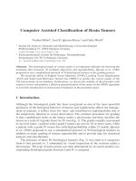
Symbolic Representation of Time Series:
A Hierarchical Coclustering Formalization
Alexis Bondu1,2,3(B) , Marc Boull´e1,2,3 , and Antoine Cornu´ejols1,2,3
1

EDF R&D, 1 avenue du G´en´eral de Gaulle, 92140 Clamart, France

2
Orange Labs, 2 avenue Pierre Marzin, 22300 Lannion, France

3
AgroParisTech, 16 rue Claude Bernard, 75005 Paris, France


Abstract. The choice of an appropriate representation remains crucial
for mining time series, particularly to reach a good trade-off between
the dimensionality reduction and the stored information. Symbolic representations constitute a simple way of reducing the dimensionality by

turning time series into sequences of symbols. SAXO is a data-driven
symbolic representation of time series which encodes typical distributions of data points. This approach was first introduced as a heuristic
algorithm based on a regularized coclustering approach. The main contribution of this article is to formalize SAXO as a hierarchical coclustering approach. The search for the best symbolic representation given
the data is turned into a model selection problem. Comparative experiments demonstrate the benefit of the new formalization, which results in
representations that drastically improve the compression of data while
keeping useful information for classification tasks.
Keywords: Time series

1

· Symbolic representation · Coclustering

Introduction

The choice of the representation of time series remains crucial since it impacts
the quality of supervised and unsupervised analysis [1]. Time series are particularly difficult to deal with due to their inherently high dimensionality when
they are represented in the time-domain [2,3]. Virtually all data mining and
machine learning algorithms scale poorly with the dimensionality. During the
last two decades, numerous high level representations of time series have been
proposed to overcome this difficulty. The most commonly used approaches are:
the Discrete Fourier Transform [4], the Discrete Wavelet Transform [5,6], the
Discrete Cosine Transform [7], the Piecewise Aggregate Approximation (PAA)
[8]. Each representation of time series encodes some information derived from
the raw data1 . According to [1], mining time series heavily relies on the choice of
1

“Raw data” designates a time series represented in the time-domain by a vector of
real values.

c Springer International Publishing Switzerland 2016

A. Douzal-Chouakria et al. (Eds.): AALTD 2015, LNAI 9785, pp. 3–16, 2016.
DOI: 10.1007/978-3-319-44412-3 1


4

A. Bondu et al.

a representation and a similarity measure. Our objective is to find a compact
and informative representation which is driven by the data. The symbolic representations constitute a simple way of reducing the dimensionality of the data
by turning time series into sequences of symbols [9]. In such representations, each
symbol corresponds to a time interval and encodes information which summarize
the related sub-series. Without making hypothesis on the data, such a representation does not allow one to quantify the loss of information. This article focuses
on a less prevalent symbolic representation which is called SAXO2 . This approach
optimally discretizes the time dimension and encodes typical distributions3 of
data points with the symbols [10]. SAXO offers interesting properties. Since this
representation is based on a regularized Bayesian coclustering4 approach called
MODL5 [11], a good trade-off is naturally reached between the dimensionality
reduction and the information loss. SAXO is a parameter-free and data-driven
representation of time series. In practice, this symbolic representation proves to
be highly informative for training classifiers. In [10], SAXO was evaluated on
public datasets and favorably compared with the SAX representation.
Originally, SAXO was defined as a heuristic algorithm. The two main contributions of this article are: (i) the formalization of SAXO as a hierarchical
coclustering approach; (ii) the evaluation of its compactness in terms of coding length and its informativeness for classification tasks. The most probable
SAXO representation given the data is defined by minimizing the new evaluation
criterion. Our objective is to yield better SAXO representations, which improve
the compression of time series while preserving the advantage of coding typical
distributions. This article is organized as follows. Section 2 briefly introduces the
symbolic representations of time series and presents the original SAXO heuristic
algorithm. Section 3 formalizes the SAXO approach resulting in a new evaluation criterion which is the main contribution of this article. Experiments are

conducted in Sect. 4 on real datasets in order to compare the SAXO evaluation
criterion with that of the MODL coclustering approach. Lastly, perspectives and
future works are discussed in Sect. 5.

2

Related Work

Numerous compact representations of time series deal with the curse of dimensionality by discretizing the time and by summarizing the sub-series within
each time interval. For instance, the Piecewise Aggregate Approximation (PAA)
encodes the mean values of data points within each time interval. The Piecewise
Linear Approximation (PLA) [12] is an other example of compact representation which encodes the gradient and the y-intercept of a linear approximation
2
3
4
5

SAXO Symbolic Aggregate approXimation Optimized by data.
The SAXO approach produces clusters of time series within each time interval which
correspond to the symbols.
The coclustering problem consist in reordering rows and columns of a matrix in
order to satisfy a homogeneity criterion.
Minimum Optimized Description Length.


Symbolic Representation of Time Series

5

of sub-series. In both cases, the representation consist of numerical values which

describe each time interval. In contrast, the symbolic representations characterize the time intervals by categorical variables [9]. For instance, the Shape
Definition Language (SDL) [13] encodes the shape of sub-series by symbols.
The SAX Approach. The Symbolic Aggregate approXimation approach is one of
the main symbolic representations of time series. It provides a distance measure
that lower bounds the Euclidian distance defined in the time-domain. This approach consists of two steps: (i) time discretization using PAA; (ii) discretization
of the outcome mean values into symbols. First, the PAA transform reduces
the dimensionality of the original time series S = {x1 , ..., xm∗ } by considering a
vector S¯ = {x¯1 , ..., x¯w } of w mean values (w < m∗ ) calculated on regular time
intervals. Then, the SAX approach discretizes the mean values {x¯i } obtained
from the PAA transform into a set of α equiprobable symbols. The interval of
values corresponding to each symbol can be analytically calculated under the
assumption that the time series have a Gaussian distribution [9]. An alternative
method consists in empirically calculating the quantiles of values in the dataset.
Figure 1 plots an example of SAX transform based on a set of three symbols (i.e. {a, b, c}). The left part of this figure illustrates that the distribution
of values is supposed to be known, and is divided into equiprobable intervals
corresponding to each symbol. Then, these intervals are exploited to discretize
the mean values into symbols within each time interval. The concatenation of
symbols baabccbc constitutes the SAX representation of the original time series.
The SAX representation has become an essential tool for time series data mining. This approach has been exploited to implement various tasks on large time
series datasets, including similarity clustering [14], anomaly detection [15,16],
discovery of motifs [17], visualization [18], stream processing [9]. Originally, the
SAX approach was designed for indexing very large sets of time series [19], and
remains a reference in this field.
The symbolic representations appear to be really helpful for processing
large datasets of time series owing to dimensionality reduction. However, these
approaches suffer several limitations.
– Most of these representations are lossy compression approaches unable to
quantify the loss of information without strong hypothesis on the data.
– The discretization of the time dimension into regular intervals is not data driven.
– The symbols have the same meaning over time irrespectively of their rank

(i.e. the ranks of the symbols may be used to improve the compression).

Fig. 1. Example of SAX representation.


6

A. Bondu et al.

– Most of these representations involve user parameters which affect the stored
information (ex: for the SAX representation, the number of time intervals and
the size of the alphabet must be specified).
The SAXO approach overcomes these limitations by optimizing the time
discretization, and by encoding typical distributions of data points within each
time interval [10]. SAXO was first defined as a heuristic which exploits the MODL
coclustering approach.
Figure 2 provides an overview of this approach by illustrating the main steps
of the learning algorithm. The joint distribution of the identifiers of the time
series C, the values X, and the timestamp T is estimated by a trivariate coclustering model. The time discretization resulting from the first step is retained,
and the joint distribution of X and C is estimated within each time interval
by using a bivariate coclustering model. The resulting clusters of time series are
characterized by piecewise constant distributions of values and correspond to the
symbols. A specific representation allows one to re-encode the time series as a
sequence of symbols. Then, the typical distribution that best represents the data
points of the time series is selected within each time interval. Figure 3(a) plots
an example of recoded time series. The original time series (represented by the
blue curve) is recoded by the “abba” SAXO word. The time is discretized into
four intervals (the vertical red lines) corresponding to each symbol. Within time
intervals, the values are discretized (the horizontal green lines): the number of
intervals of values and their locations are not necessary the same. The symbols

correspond to typical distributions of values: conditional probabilities of X are
associated with each cell of the grid (represented by the gray levels); Fig. 3b gives
an example of the alphabet associated with the second time interval. The four
available symbols correspond to typical distributions which are both represented
by gray levels and by histograms. By considering Figs. 3a and b, b appears to
be the closest typical distribution of the second sub-series.
As in any heuristic approach, the original algorithm finds a suboptimal solution for selecting the most suitable SAXO representation given the data. Solving
this problem in an exact way appears to be intractable, since it is comparable
to the coclustering problem which is NP-hard. The main contribution of this
paper is to formalize the SAXO approach within the MODL framework. We
claim this formalization is a first step to improving the quality of the SAXO
representations learned from data. In this article, we define a new evaluation

Fig. 2. Main steps of the SAXO learning algorithm.


Symbolic Representation of Time Series

(a)

7

(b)

Fig. 3. Example of a SAXO representation (a) and the alphabet of the second time
interval (b). (Color figure online)

criterion denoted by Csaxo (see Sect. 3). The most probable SAXO representation given the data is defined by minimizing Csaxo . We expect to reach better
representations by optimizing Csaxo , instead of exploiting the original heuristic
algorithm.

3

Formalization of the SAXO Approach

This section presents the main contribution of this article: the SAXO approach is formalized as a hierarchical coclustering approach. As illustrated in
Fig. 4, the originality of the SAXO approach is that the groups of identifiers
(variable C) and the intervals of values (variable X) are allowed to change over
time. By contrast, the MODL coclustering approach forces the discretization of
C and X to be the same within time intervals. Our objective is to reach better
models by removing this constraint.
A SAXO model is hierarchically instantiated by following two successive
steps. First, the discretization of time is determined. The bivariate discretization C × X is then defined within each time interval. Additional notations are
required to describe the sequence of bivariate data grids.
X

X

MODLcoclustering

SAXO

T
C

T

C

Fig. 4. Examples of a MODL coclustering model (left part) and a SAXO model (right

part).


8

A. Bondu et al.

Notations for time series: In this article, the input dataset D is considered to be a collection of N time series denoted Si (with i ∈ [1, N ]). Each
time series consists of mi data points, which are couples of values X and
N
timestamps T . The total number of data points is denoted by m = i=1 mi .
Notations for the t-th time interval of a SAXO model:
–
–
–
–
–
–
–
–
–
–

kT : number of time intervals;
t
kC
: number of clusters of time series;
t
: number of intervals of value;
kX

kC (i, t) : index of the cluster that contains the sub-series of Si ;
{ntiC } : number of time series in each cluster itC ;
mt : number of data point;
mti : number of data points of each time series Si ;
mtiC : number of data points in each cluster itC ;
{mtjX } : number of data points in the intervals jX ;
{mtiC jX } : number of data points belonging to each cell (iC , jX ).

Eventually, a SAXO model M is first defined by a number of time intervals
and the location of their bounds. The bivariate data grids C × X within each
time interval are defined by: (i) the partition of the time series into clusters; (ii)
the number of intervals of values; (iii) the distribution of the data points on the
cells of the data grid; (iv) for each cluster, the distribution of the data points
on the time series belonging to the same cluster. Section 3.1 presents the prior
distribution of the SAXO models. The likelihood of a SAXO model given the
data is described in Sect. 3.2. A new evaluation criterion which defines the most
probable model given the data is proposed in Sect. 3.3.
3.1

Prior Distribution of the SAXO Models

The proposed prior distribution P (M ) exploits the hierarchy of the parameters
of the SAXO models and is uniform at each level. The prior distribution of the
number of time intervals kT is given by Eq. 1. The parameter kT belongs to [1, m],
with m representing the total number of data points. All possible values of kT
are considered as equiprobable. By using combinatorics, the numbutation [13]. It is based upon the calculation of an envelope; however this calculation is not trivially transferable to the case of multidimensional
time series simply by generalizing the uni-dimensional equations. Thus, we will
unfortunately not consider it in our study.
However, a cheap bound can be evaluated several times as DTW progresses as
follows: for any row i, the minimum of all cells A[i,.] is a lower bound to the DTW

result. Indeed, this result is the last cell of the last row, and the sequence mapping
a row i to minj A[i,j] is increasing, because the costs are positive. Hence, during
each outer loop iteration (i.e., on index i), we can store the minimum of the
current row and compare it to the best-so-far for possibly early abandoning. This
can be transposed directly to Coarse-DTW without additional modifications.

6

Kernelization of CoarseDTW

Besides the fact that DTW and CoarseDTW are not metrics (they do not comply
with the triangle inequality), it is furthermore not possible to directly derive a
positive definite kernel from such elastic distances. Hence, their use in kernel
approaches such as Support Vector Machines (SVM) is questionable and the
experience shows that directly substituting DTW into a Gaussian kernel, for
instance, does not lead to satisfactory results [18].


166

M. Dupont and P.-F. Marteau

Recent works [7,18] propose new guidelines to regularize kernels constructed
from elastic measures similar to DTW. Following the line of regularization
proposed in [18], an instance of positive definite kernel deriving from the
CoarseDTW (Kcdtw ) measure can be translated into the Algorithm 4, which
relies on two recursive terms, namely Kxy and Kxx .
The main idea behind this line of regularization is to replace the operators
min and max (which prevent the symmetrization of the kernel) by a summation
operator ( ). This leads to consider, not only the best possible alignment, but

also all good (or nearly best) paths by summing up their overall cost. The parameter ν is used to control what we mean by a good alignment, thus penalizing
more or less alignments too far from the optimal ones. This parameter can be
easily optimized through a cross-validation.
The proof for the positive definiteness of Kcdtw is very similar to the one
given in [18] for the regularized DTW kernel, except that the local kernels
2
e−ν·ξ(s(p),t(q))·δE (v(p),w(q)) , where ξ(s(p), t(q)) stands for s(p), t(q) or φ(s(p), t(q))
should be understood as a positive definite kernel defined on the set of constant
time series of varying lengths. Note that if the two time series in argument are
not sparse (this is the case when no downsampling is applied), the Kcdtw kernel
corresponds exactly to the regularized DTW kernel described in [18].
Algorithm 4 is based on the following conventions: ∀p ≥ 0, if p > m = |(s, v)|
then s(p) = s(m) and v(p) = v(m) and similarly ∀q ≥ 0, if q > n = |(t, w)| then
t(q) = s(n) and v(q) = v(n).

Algorithm 4. KCoarse-DTW
1: procedure KCoarse-DTW((s, v), (t, w))
2:
Kxy = new matrix [0..n, 0..m]
3:
Kxx = new matrix [0..n, 0..m]
4:
Kxy [0, .] = Kxy [., 0] = 0 and Kxy [0, 0] = 1.0
5:
Kxx [0, .] = Kxx [., 0] = 0 and Kxx [0, 0] = 1.0
6:
for i = 1 to n do
7:
for j = 1 to m do
8:

Kxy [i, j] = 13 ( exp(−ν.si .δ(vi , wj )) · Kxy [i−1, j]+
9:
exp(−ν.ti .δ(vi , wj )) · Kxy [i, j −1]+
10:
exp(−ν.φ(si , tj ).δ(vi , wj )) · Kxy [i−1, j −1] )
11:
if i < m and j < n then
12:
Kxx [i, j] = 13 ( exp(−ν.si .δ(vi , wi )) · Kxx [i−1, j]+
13:
exp(−ν.ti .δ(vi , wi )) · Kxx [i, j −1] )
14:
if i == j then
15:
Kxx [i, j] + = 13 exp(−ν.φ(si , ti ).δ(vi , wi )) · Kxx [i−1, j −1]
16:
return Kxy [n, m] + Kxx [n, m]

6.1

Normalization of KCoarse-DTW

As KCoarse-DTW (in short Kcdtw ) evaluates the sum on all possible alignment
2
paths of the products of local alignment costs e−ν·ξ(s(p),t(q))·δE (v(p),w(q)) ≤ 1,


Coarse-DTW for Sparse Time Series Alignment

167

its values can be very small depending on the size of the time series and the
selected value for ν. Hence, Kcdtw values tend to 0 when ν tends towards ∞,
except when the two compared time series are identical (the corresponding Gram
matrix suffers from a diagonal dominance problem). As proposed in [18], a manner to avoid numerical troubles consists in using the following normalized kernel:
˜ cdtw (., .) = exp α log(Kcdtw (., .)) − log(min(Kcdtw ))
K
log(max(Kcdtw )) − log(min(Kcdtw ))
where max(Kcdtw ) and min(Kcdtw ) respectively are the max and min values
taken by the kernel on the learning dataset and α > 0 a positive constant (α = 1
by default). If we forget the proportionality constant, this leads to take the
kernel Kcdtw at a power τ = α/(log(max(Kcdtw )) − log(min(Kcdtw ))), which
˜ cdtw ∝ K τ
shows that the normalized kernel K
cdtw is still positive definite ([3],
Proposition 2.7).

7
7.1

Results
DTW vs. Coarse-DTW in 1-NN Classification

In this first setup we considered the classification accuracy and speed of various
labeled time series datasets. The classifier is 1-NN and we enabled all optimizations described earlier that apply to multidimensional time series, namely: early
abandoning on LBKim and early abandoning on the minima of rows. The disd
tance chosen is the squared version, δ(x, y) = x − y 22 = s=1 (xs − ys )2 . We
report only the classification time, not the learning time.
Dataset MSRAction3D [16] consists of 10 actors executing the same gestures
several times, with 60 dimensions (twenty 3D joints). To classify this dataset,

we cross-validated all possible combinations of 5 actors in training and 5 in test,
thus totaling 252 rounds.
The dataset uWaveGestureLibrary [XYZ] comes from the UCR time series
database [11]. It can be considered as three independent uni-dimensional
datasets, but we rather used it here as a single set of 3-dimensional time series.
The interest is obvious: in 1-NN DTW classification, we went from individual
1D errors of respectively 27.3 %, 36.6 % and 34.2 %, down to only 2.8 % when
the three time series sets are taken together.
Finally, for the sake of comparison, we also ran our tests on the other UCR
time series datasets at our disposal. It should be noted that they are all unidimensional, however we exclusively considered them as multidimensional time
series which happen to have a dimension of d = 1. This means in particular that
some of the traditional lower bounds such as LBKeogh cannot be used, only the
multidimensional-enabled ones described earlier.
For each dataset, we ran the classification once with DTW to obtain a reference value both time- and accuracy-wise. Then, we ran Coarse-DTW, with
several values of ρ, as follows: the dense time series are first downsampled with
Bubble into sparse time series, according to the current ρ, and then classified


168

M. Dupont and P.-F. Marteau

Fig. 5. 1-NN classification time and error rate of Coarse-DTW as ρ increases. For
reference, DTW results are shown as horizontal bars (independent of ρ).

with Coarse-DTW. The time and error rate was measured at every run. In Fig. 5
we show the full results for a few datasets.
A general trend can be observed (Fig. 5): as ρ increases, classification time
decreases. However, this comes at the expense of a higher error rate. This is
expected: indeed, downsampled time series contain less information than their

dense counterparts. Now, we can observe that some time series allow ρ to increase
quite a bit (and therefore classification goes much faster) before the accuracy
really degrades.
In order to quantify this effect, we proceed as follows. We first set a threshold
on the error rate. Here, we select the threshold to be 2 % (absolute error) above
our reference, the DTW error rate. (For example, if the DTW error rate were
27.1 %, we would set the threshold at 29.1 %, which might or might not be
acceptable depending on the user’s constraints.) Then we find the value of
ρ∗ = max{ρ | ∀ρ ≤ ρ, errρ ≤ errDTW + 2 %}

(4)

which represents the last acceptable value before the error rates first goes above
the threshold (the “breakout”). The CPU time associated with the run of ρ∗ is
likely to be below the DTW CPU time, which is why we define the speedup as
their ratio:
CPU time DTW
speedup =
(5)
CPU time Coarse-DTW at ρ∗
Furthermore, we tested each of the three possibilities for φ. Of all three, we
selected only the ρ∗ value giving the best time. The values of ρ∗ and the speedup
are summarized in Table 1, along with the winning φ.


Coarse-DTW for Sparse Time Series Alignment

169

Table 1. Performance of Coarse-DTW (for a threshold at +2 % abs. err.) compared

to DTW, in 1-NN classification (datasets from [11, 16]).
Dataset

d

Time DTW Time Coarse-DTW Speedup Best φ

3

1850 s

0.769 s

2413.3x φstairs

60

1710 s

428 s

4.0x

φmax

Adiac

1

21.0 s

13.0 s

1.6x

φstairs

Beef

1

1.35 s

0.014 s

93.5x

φmax

CBF

1

3.18 s

0.0393 s

80.9x

φdiag

ChlorineConcentration

1

73.2 s

14.0 s

5.2x

φmax

CinC ECG torso

1

1690 s

0.413 s

4100.7x φmax

Coffee

1

0.479 s

0.139 s

3.5x

DiatomSizeReduction

1

3.81 s

0.241 s

15.8x

φmax

ECG200

1

0.258 s

0.012 s

20.7x

φmax

uWaveGestureLibrary [XYZ]
MSRAction3D

φmax

ECGFiveDays

1

2.34 s

0.283 s

8.2x

φmax

FaceAll

1

73.3 s

21.5 s

3.4x

φmax

FaceFour

1

2.69 s

0.031 s

85.8x

φstairs

FacesUCR

1

42.7 s

7.46 s

5.7x

φmax

FISH

1

47.1 s

38.0 s

1.2x

φmax

Gun Point

1

0.653 s

0.108 s

6.1x

φdiag

Haptics

1

445 s

0.860 s

516.7x

φmax

InlineSkate

1

1790 s

0.548 s

3276.1x φdiag

ItalyPowerDemand

1

0.236 s

0.103 s

2.3x

φstairs

Lighting2

1

17.0 s

0.440 s

38.6x

φstairs

Lighting7

1

4.66 s

5.21s

0.9x

φmax

MALLAT

1

1460 s

6.408 s

228.4x

φmax

MedicalImages

1

2.92 s

0.261 s

11.2x

φmax

MoteStrain

1

1.14 s

0.0480 s

23.7x

φmax

NonInvasiveFetalECG Thorax1

1

9820 s

516 s

19.0x

φmax

NonInvasiveFetalECG Thorax2

1

9720 s

310 s

31.3x

φmax

OliveOil

1

3.15 s

1.43 s

2.2x

φdiag

OSULeaf

1

59.3 s

2.16 s

27.4x

φstairs

SonyAIBORobot Surface

1

0.465 s

0.245 s

1.9x

φmax

SonyAIBORobot SurfaceII

1

0.902 s

0.150 s

6.0x

φstairs

StarLightCurves

1

44700 s

58.6 s

763.0x

φmax

SwedishLeaf

1

19.0 s

11.5 s

1.7x

φmax

Symbols

1

21.8 s

1.91 s

11.4x

φmax

synthetic control

1

1.97 s

0.624 s

3.2x

φmax

Trace

1

2.36 s

0.00636 s

371.3x

φmax

TwoLeadECG

1

0.827 s

0.0869 s

9.5x

φmax

Two Patterns

1

371 s

0.668 s

556.4x

φmax

wafer

1

158 s

0.402 s

392.1x

φmax

WordsSynonyms

1

87.4 s

4.61 s

18.9x

φmax

yoga

1

581 s

4.78 s

121.7x

φmax

170

M. Dupont and P.-F. Marteau

Additionally, our study aimed to search for the best φ function for the diagonal weight. We can conclude from Table 1 that the most satisfactory is φmax ,
offering the best ratio accuracy/time. Actually, it appears from our experience
that φdiag was good enough accuracy-wise but was too slow due to the square
root. Thus, we recommend selecting φmax by default.
7.2

SVM Classification with KCoarse-DTW

We also tested the accuracy of our regularized version, KCoarse-DTW, normalized as described in Sect. 6.1, with different values of ρ to see how accuracy
degrades with approximation.

Fig. 6. SVM classification time and error rate of our regularized kernel, KCoarse-DTW.
For reference, 1-NN DTW results are shown as horizontal bars (top: CPU time, bottom:
error rate).

With KCoarse-DTW and with very small values of ρ, we are in general able
to outperform 1-NN DTW. We must add that this was not the case for all time
series when ρ increases, so this really depends on the nature of the time series
in question.
In Fig. 6, we present two datasets where the regularized kernel performed
better. (For FaceFour, the same (C, σ) was found for ρ = 0 and reused afterwards,
whereas on CinC ECG Torso, there was a new grid search for each ρ.) The
behavior is comparable to 1-NN classification with Coarse-DTW, except we start
at ρ = 0 with a lower error rate. Then accuracy degrades as expected. SVM
takes usually more time to run than 1-NN, but KCoarse-DTW helps by making

it possible to decrease the classification time.

8

Conclusions

Not only have we transposed DTW into Coarse-DTW, a version accepting sparse
time series, but we have also developed Bubble, an extremely efficient, streamable algorithm to generate such sparse time series from regular ones. By coupling
those two mechanisms, we were able to discover that time series can be classified much faster in nearest-neighbor classification; the user can reach the desired
tradeoff between speed and accuracy, by tuning the parameter ρ in the downsampling algorithm. Some time series are far more subject to downsampling than


Coarse-DTW for Sparse Time Series Alignment

171

others, and therefore results can differ depending on which context time series
originate. For example, smooth time series like gestures present a considerable
ability to be downsampled, producing good results in classification speedup.
We also explored the regularization of Coarse-DTW, for use as an SVM kernel. For some time series, results were encouraging, giving classification results
much better than 1-NN. As it was expected, the accuracy degraded as the downsampling radius ρ increased, giving once again the user the ability to choose a
suitable tradeoff between speed and accuracy.
Coarse-DTW and Bubble have a great potential to be used in a variety
of scenarios beyond offline classification; for example, they are totally suitable
to reduce time series storage space, or also to reconize learnt patterns within
a multidimensional stream. Finally, in an embedded context, where energy is
scarce, the speedup offered by Coarse-DTW can also be interpreted as a saving
in CPU cycles, which can be tremendously helpful.
Acknowledgements. This study was co-funded by the ANRT agency and Thales
Optronique SAS, under the PhD CIFRE convention 2013/0932.

References
1. Al-Naymat, G., Chawla, S., Taheri, J.: Sparsedtw: a novel approach to speed up
dynamic time warping. In: Proceedings of the Eighth Australasian Data Mining Conference, AusDM 2009, Darlinghurst, Australia, vol. 101, pp. 117–127.
Australian Computer Society Inc., Australia (2009)
2. Apostolico, A., Landau, G.M., Skiena, S.: Matching for run-length encoded strings.
In: 1997 Proceedings of the Compression and Complexity of Sequences, pp. 348–356,
June 1997
3. Berg, C., Christensen, J.P.R., Ressel, P.: Harmonic Analysis on Semigroups: Theory of Positive Definite and Related Functions. Graduate Texts in Mathematics,
vol. 100. Springer, New York (1984)
4. Chakrabarti, K., Keogh, E., Mehrotra, S., Pazzani, M.: Locally adaptive dimensionality reduction for indexing large time series databases. ACM Trans. Database
Syst. 27(2), 188–228 (2002)
5. Chen, L., Ng, R.: On the marriage of Lp-norm and edit distance. In: Proceedings of
the 30th International Conference on Very Large Data Bases, pp. 792–801 (2004)
6. Chu, S., Keogh, E.J., Hart, D.M., Pazzani, M.J.: Iterative deepening dynamic
time warping for time series. In: Grossman, R.L., Han, J., Kumar, V., Mannila,
H., Motwani, R. (eds.) Proceedings of the Second SIAM International Conference
on Data Mining, Arlington, VA, USA, 11–13 April 2002, pp. 195–212. SIAM (2002)
7. Cuturi, M., Vert, J.-P., Birkenes, O., Matsui, T.: A kernel for time series based on
global alignments. In: IEEE ICASSP 2007, vol. 2, pp. II-413–II-416, April 2007
8. Fr´echet, M.: Sur Quelques Points du Calcul Fonctionnel. Th`ese, Facult´e des Sciences de Paris (1906)
9. Gudmundsson, S., Runarsson, T.P., Sigurdsson, S.: Support vector machines and
dynamic time warping for time series. In: 2008 IEEE International Joint Conference on Neural Networks, IJCNN 2008. IEEE World Congress on Computational
Intelligence, pp. 2772–2776, June 2008


172

M. Dupont and P.-F. Marteau

10. Itakura, F.: Minimum prediction residual principle applied to speech recognition.
IEEE Trans. Acoust. Speech Sig. Process. 23(1), 67–72 (1975)
11. Keogh, E.J., Xi, X., Wei, L., Ratanamahatana, C.A.: The UCR time
series classification-clustering datasets (2006). />time series data/
12. Keogh, E., Chakrabarti, K., Pazzani, M., Mehrotra, S.: Dimensionality reduction
for fast similarity search in large time series databases. J. Knowl. Inf. Syst. 3,
263–286 (2000)
13. Keogh, E., Ratanamahatana, C.A.: Exact indexing of dynamic time warping.
Knowl. Inf. Syst. 7(3), 358–386 (2005)
14. Keogh, E.J., Pazzani, M.J.: Scaling up dynamic time warping for datamining applications. In: Proceedings of the Sixth ACM SIGKDD International Conference on
Knowledge Discovery and Data Mining, KDD 2000, pp. 285–289. ACM, New York,
NY, USA (2000)
15. Lemire, D.: Faster retrieval with a two-pass dynamic-time-warping lower bound.
Pattern Recogn. 42(9), 2169–2180 (2009)
16. Li, W., Zhang, Z., Liu, Z.: Action recognition based on a bag of 3D points. In:
Proceedings of IEEE International Workshop on CVPR for Human Communicative
Behavior Analysis, pp. 9–14. IEEE CS Press (2010)
17. Marteau, P.F.: Time warp edit distance with stiffness adjustment for time series
matching. IEEE Trans. Pattern Anal. Mach. Intell. 31(2), 306–318 (2008)
18. Marteau, P.-F., Gibet, S.: On recursive edit distance kernels with application to
time series classification. IEEE Trans. Neural Netw. Learn. Syst., 1–14 (2014)
19. Marteau, P.-F., Gibet, S., Reverdy, C.: Down-Sampling coupled to elastic kernel
machines for efficient recognition of isolated gestures. In: International Conference
on Pattern Recognition, ICPR 2014, pp. 336–368. IEEE, Stockholm, Sweden, August
2014
20. Patel, P., Keogh, E., Lin, J., Lonardi, S.: Mining motifs in massive time series databases. In: Proceedings of IEEE International Conference on Data Mining, ICDM
2002, pp. 370–377 (2002)
21. Sakoe, H., Chiba, S.: A dynamic programming approach to continuous speech
recognition. In: Proceedings of the 7th International Congress of Acoustic,
pp. 65–68 (1971)

22. Sakurai, Y., Yoshikawa, M., Faloutsos, C.: FTW: Fast similarity search under the
time warping distance. In: Proceedings of the Twenty-Fourth ACM SIGMODSIGACT-SIGART Symposium on Principles of Database Systems, PODS 2005,
pp. 326–337. ACM, New York, NY, USA (2005)
23. Salvador, S., Chan, P.: Toward accurate dynamic time warping in linear time and
space. Intell. Data Anal. 11(5), 561–580 (2007)
24. Shou, Y., Mamoulis, N., Cheung, D.W.: Fast and exact warping of time series using
adaptive segmental approximations. Mach. Learn. 58(2–3), 231–267 (2005)
25. Velichko, V.M., Zagoruyko, N.G.: Automatic recognition of 200 words. Int. J. ManMach. Stud. 2, 223–234 (1970)
26. Kim, S.W., Park, S., Chu, W.W.: An index-based approach for similarity search
supporting time warping in large sequence databases. In: ICDE, pp. 607–614 (2001)
27. Yi, B.-K., Faloutsos, C.: Fast time sequence indexing for arbitrary Lp norms. In:
Proceedings of the 26th International Conference on Very Large Data Bases, VLDB
2000, pp. 385–394. Morgan Kaufmann Publishers Inc., San Francisco, CA, USA
(2000)


Author Index

Andrade-Pacheco, Ricardo

95

Bailly, Adeline 17
Bondu, Alexis 3
Boullé, Marc 3
Camps-Valls, Gustau 78
Chapel, Laetitia 17
Cornuéjols, Antoine 3
Do, Cao-Tri 131
Douzal-Chouakria, Ahlame

Dupont, Marc 157
Fortunati, Luigi

Malinowski, Simon 17
Marié, Sylvain 131
Marteau, Pierre-François
Mateo, Fernando 78
Micheli, Alessio 65
Mubangizi, Martin 95
Muñoz-Marí, Jordi 78
Nelson, James D.B.

131, 144

Parodi, Oberdan 65
Pedrelli, Luca 65
Quinn, John

65

111

95

Rombaut, Michèle

131

Gallicchio, Claudio 65
Gaussier, Eric 144

Gibberd, Alex J. 111
Guyet, Thomas 17

Soheily-Khah, Saeid 144
Spiegel, Stephan 31

Jain, Brijnesh

Tavenard, Romain

31

Lafuente-Rego, Borja
Laparra, Valero 78
Lawrence, Neil 95

49

17

Verrelst, Jochem 78
Vilar, Jose A. 49
Vozzi, Federico 65

157