Psychophysics a practical introduction 2nd ed

PSYCHOPHYSICS
A PRACTICAL INTRODUCTION
SECOND EDITION
FREDERICK A.A. KINGDOM
McGill University, Montreal, Quebec, Canada

NICOLAAS PRINS
University of Mississippi, Oxford, MS, USA

AMSTERDAM • BOSTON • HEIDELBERG • LONDON
NEW YORK • OXFORD • PARIS • SAN DIEGO
SAN FRANCISCO • SINGAPORE • SYDNEY • TOKYO
Academic Press is an imprint of Elsevier


Academic Press is an imprint of Elsevier
125 London Wall, London EC2Y 5AS, UK
525 B Street, Suite 1800, San Diego, CA 92101-4495, USA
225 Wyman Street, Waltham, MA 02451, USA
The Boulevard, Langford Lane, Kidlington, Oxford OX5 1GB, UK
Copyright © 2016, 2010 Elsevier Ltd. All rights reserved.
Cover image: This item is reproduced by permission of The Huntington Library, San Marino, California.
No part of this publication may be reproduced or transmitted in any form or by any means, electronic or mechanical,
Including photocopying, recording, or any information storage and retrieval system, without permission in writing from
the publisher. Details on how to seek permission, further information about the Publisher’s permissions policies and our
arrangements with organizations such as the Copyright Clearance Center and the Copyright Licensing Agency, can be
found at our website: www.elsevier.com/permissions.
This book and the individual contributions contained in it are protected under copyright by the Publisher (other than
as may be noted herein).

Notices

Knowledge and best practice in this field are constantly changing. As new research and experience broaden our
understanding, changes in research methods, professional practices, or medical treatment may become necessary.
Practitioners and researchers must always rely on their own experience and knowledge in evaluating and using any
information, methods, compounds, or experiments described herein. In using such information or methods they should
be mindful of their own safety and the safety of others, including parties for whom they have a professional
responsibility.
To the fullest extent of the law, neither the Publisher nor the authors, contributors, or editors, assume any liability for
any injury and/or damage to persons or property as a matter of products liability, negligence or otherwise, or from any
use or operation of any methods, products, instructions, or ideas contained in the material herein.
ISBN: 978-0-12-407156-8
British Library Cataloguing-in-Publication Data
A catalogue record for this book is available from the British Library
Library of Congress Cataloging-in-Publication Data
A catalog record for this book is available from the Library of Congress
For information on all Academic Press publications
visit our website at />
Publisher: Mica Haley
Acquisition Editor: Melanie Tucker
Editorial Project Manager: Kristi Anderson
Production Project Manager: Caroline Johnson
Designer: Matt Limbert
Typeset by TNQ Books and Journals
www.tnq.co.in
Printed and bound in the United States of America


Dedication
FK would like to dedicate this book to his late parents Tony and Joan, and present
family Beverley and Leina. NP would like to dedicate this book to his mother Nel and late
father Arie.

About the Authors
Frederick A.A. Kingdom is a Professor at McGill University conducting research into
various aspects of visual perception, including color vision, brightness perception, stereopsis,
texture perception, contour-shape coding, the perception of transparency, and visual illusions. He also has an interest in models of summation for the detection of multiple stimuli.
Nicolaas Prins is an Associate Professor at the University of Mississippi specializing in
visual texture perception, motion perception, contour-shape coding, and the use of statistical
methods in the collection and analysis of psychophysical data.

ix


Preface to the Second Edition
comparisons. We have also provided an
updated quick reference guide to the terms,
concepts, and many of the equations
described in the book.
In writing the second edition we have
endeavored to improve each chapter and
have extended all the technical chapters to
include new procedures and analyses.
Chapter 7 is the book’s one new chapter. It
deals with an old but vexing question of
how multiple stimuli combine to reach
threshold. The chapter attempts to derive
from first principles and make accessible to
the reader the mathematical basis of the
myriads of summation models, scenarios,
and metrics that are scattered throughout

the literature.
Writing both editions of this book has
been a considerable challenge for its authors.
Much effort has been expended in trying to
make accessible the theory behind different
types of psychophysical data analysis. For
those psychophysical terms that to us did
not appear to have a clear definition we have
improvised our own (e.g., the definition of
“appearance” given in Chapter 2), and for
other terms where we felt there was a lack of
clarity we have challenged existing convention (e.g., by referring to a class of forcedchoice tasks as 1AFC). Where we have
challenged convention we have explained
our reasoning and hope that even if readers
do not agree with us, they will still find our
ideas on the matter thought-provoking.

The impetus for this book was a recurring
question: “Is there a book that explains how
to do psychophysics?” Evidently, a book was
needed that not only explained the theory
behind psychophysical procedures but also
provided the practical tools necessary for
their implementation. What seemed to be
missing was a detailed and accessible exposition of how raw psychophysical responses
are turned into meaningful measurements of
sensory function; in other words, a book that
dealt with the nuts and bolts of psychophysics data analysis.
The need for a practical book on psychophysics inevitably led to a second need: a
comprehensive package of software for

analyzing psychophysical data. The result
was Palamedes. Initially developed in
conjunction with the first edition of the book,
Palamedes has since taken on a life of its
own, and one purpose of the second edition
is to catch up with its latest developments!
Palamedes will of course continue to be
developed so readers are encouraged to keep
an eye on the regular updates.
The first few chapters of the book are
intended to introduce the basic concepts and
terminology of psychophysics as well as
familiarize readers with a range of psychophysical procedures. The remaining chapters
focus on specialist topics: psychometric
functions, adaptive procedures, signal
detection theory, summation measures,
scaling methods, and statistical model

xi


Acknowledgments
We are indebted to the following persons for kindly reviewing and providing insightful
comments on individual chapters: Neil Macmillan and Douglas Creelman for helping one of
the authors (FK) get to grips with the calculation of d0 for same-different tasks (Chapter 6);
Mark Georgeson for providing the derivation of the equation for the criterion measure lnb for
a 2AFC task (Chapter 6); Alex Baldwin for the idea of incorporating a stimulus scaling factor
g for converting stimulus intensity to d0 when modeling psychometric functions within a
Signal Detection Theory framework (Chapters 6 and 7); Mark McCourt for providing the
figures illustrating grating-induction (Chapter 3); Laurence Maloney for permission to

develop and describe the routines for Maximum Likelihood Difference Scaling (Chapter 8);
Stanley Klein for encouraging us to include a section on the Chi-squared test (Chapter 9); and
Ben Jennings for carefully checking the equations in the summation chapter (Chapter 7).
Thanks also to the many personsdtoo many to mention individuallydwho have over the
years expressed their appreciation for the book as well as the Palamedes toolbox and
provided useful suggestions for improvements to both.

xiii


C H A P T E R

1
Introduction and Aims
Frederick A.A. Kingdom1, Nicolaas Prins2
1

McGill University, Montreal, Quebec, Canada; 2University of Mississippi, Oxford, MS, USA

O U T L I N E
1.1 What is Psychophysics?

1

1.2 Aims of the Book

1

1.3 Organization of the Book

2

1.4 What’s New in the Second
Edition?

5

References

9

1.1 WHAT IS PSYCHOPHYSICS?
According to the online encyclopedia Wikipedia, psychophysics “. quantitatively investigates the relationship between physical stimuli and the sensations and perceptions they
affect.” The term was first coined by Gustav Theodor Fechner, who in his Elements of Psychophysics (1860/1966) set out the principles of psychophysical measurement, describing the
various procedures used by experimentalists to map out the relationship between matter
and mind. Although psychophysics refers to a methodology, it is also a research area in its
own right, and much effort continues to be devoted to developing new psychophysical techniques and new methods for analyzing psychophysical data.
Psychophysics can be applied to any sensory system, whether vision, hearing, touch, taste,
or smell. This book primarily draws on the visual system to illustrate the principles of
psychophysics, but the principles are applicable to all sensory domains.

1.2 AIMS OF THE BOOK
Broadly speaking, the book has three aims. The first is to provide newcomers to psychophysics with an overview of different psychophysical procedures in order to help them

Psychophysics
/>
1

Copyright © 2016 Elsevier Ltd. All rights reserved.

2

1. INTRODUCTION AND AIMS

select the appropriate designs and analyses for their experiments. The second aim is to
direct readers to the software tools, in the form of Palamedes, for analyzing psychophysical
data. This is intended for both newcomers and experienced researchers alike. The third aim
is to explain the theory behind the analyses. Again both newcomers and experienced researchers should benefit from the detailed expositions of the bulk of the underlying theory.
To this end we have made every effort to make accessible the theory behind a wide range of
psychophysical procedures, analytical principles, and mathematical computations, such as
Bayesian curve fitting; the calculation of d-primes (dʹ); summation theory; maximum likelihood difference scaling; goodness-of-fit measurement; bootstrap analysis; and likelihoodratio testing, to name but a few. In short, the book is intended to be both practical and
pedagogical.
The inclusion of the description of the Palamedes tools, placed in this edition in
separate boxes alongside the main text, will hopefully offer the reader something more
than is provided by traditional textbooks, such as the excellent Psychophysics: The Fundamentals by Gescheider (1997). If there is a downside, however, it is that we do not always
delve as deeply into the relationship between psychophysical measurement and sensory
function as The Fundamentals does, except when necessary to explain a particular psychophysical procedure or set of procedures. In this regard A Practical Introduction is not
intended as a replacement for other textbooks on psychophysics but as a complement to
them, and readers are encouraged to read other relevant texts alongside our own. Two
noteworthy recent additions to the literature on psychophysics are Knoblauch and
Maloney’s (2012) Modeling Psychophysical Data in R and Lu and Dosher’s (2013) Visual
Psychophysics.
Our approach of combining the practical and the pedagogical into a single book may not
be to everyone’s taste. Doubtless some would prefer to have the description of the software
routines put elsewhere. However, we believe that by describing the software alongside the
theory, newcomers will be able to get a quick handle on the nuts and bolts of
psychophysics methods, the better to then delve into the underlying theory if and when
they choose.

1.3 ORGANIZATION OF THE BOOK
The book can be roughly divided into two parts. Chapters 2 and 3 provide an overall
framework and detailed breakdown of the variety of psychophysical procedures available
to the researcher. Chapters 4e9 are the technical chapters. They describe the theory and
implementation for six specialist topics: psychometric functions; adaptive methods;
signal detection measures; summation measures; scaling methods; and model comparisons
(Box 1.1).
In Chapter 2 we provide an overview of some of the major varieties of psychophysical
procedures and offer a framework for classifying psychophysics experiments. The approach
taken here is an unusual one. Psychophysical procedures are discussed in the context of a critical examination of the various dichotomies commonly used to differentiate psychophysics
experiments: Class A versus Class B; Type 1 versus Type 2; performance versus appearance;
forced-choice versus nonforced-choice; criterion-dependent versus criterion-free; objective


3

1.3 ORGANIZATION OF THE BOOK

BOX 1.1

PALAMEDES
According to Wikipedia, the Greek mythological figure Palamedes (“pal-uh-MEE-deez”) is
said to have invented “. counting, currency, weights and measures, jokes, dice and a forerunner of chess called pessoi, as well as military ranks.” The story goes that Palamedes also
uncovered a ruse by Odysseus. Odysseus had promised Agamemnon that he would defend
the marriage of Helen and Menelaus but pretended to be insane to avoid having to honor his
commitment. Unfortunately, Palamedes’s unmasking of Odysseus led to a gruesome end; he
was stoned to death for being a traitor after Odysseus forged false evidence against him.
Palamedes was chosen as the name for the toolbox because of the legendary figure’s (presumed) contributions to the art of measurement, interest in stochastic processes (he did invent
dice!), numerical skills, humor, and wisdom. The Palamedes Swallowtail butterfly (Papilio
palamedes) on the front cover also provides the toolbox with an attractive icon.

Palamedes is a set of routines and demonstration programs written in MATLABÒ for
analyzing psychophysical data (Prins and Kingdom, 2009). The routines can be downloaded
from www.palamedestoolbox.org. We recommend that you check the website periodically,
because new and improved versions of the toolbox will be posted there for download.
Chapters 4e9 explain how to use the routines and describe the theory behind them. The
descriptions of Palamedes do not assume any knowledge of MATLAB, although a basic
knowledge will certainly help. Moreover, Palamedes requires only basic MATLAB; the
specialist toolboxes such as the Statistics toolbox are not required. We have also tried to make
the routines compatible with earlier versions of MATLAB, where necessary including alternative functions that are called when later versions are undetected. Palamedes is also
compatible with the free software package GNU Octave ().
It is important to bear in mind what Palamedes is not. It is not a package for generating
stimuli or for running experiments. In other words it is not a package for dealing with the
“front-end” of a psychophysics experiment. The two exceptions to this rule are the Palamedes
routines for adaptive methods, which are designed to be incorporated into an actual experimental program, and the routines for generating stimulus lists for use in scaling experiments.
But by and large, Palamedes is a different category of toolbox from the stimulus-generating
toolboxes such as VideoToolbox ( PsychToolbox
(), PsychoPy (; see also Peirce, 2007, 2009),
and Psykinematix ( (for a comprehensive list of such
toolboxes see Although
some of these toolboxes contain routines that perform similar functions to some of the routines
in Palamedes, for example fitting psychometric functions (PFs), they are in general complementary to, rather than in competition with, Palamedes.
A few software packages deal primarily with the analysis of psychophysical data. Most of
these are aimed at fitting and analyzing psychometric functions. psignifit (http://psignifit.
sourceforge.net/; see also Fründ et al., 2011) is perhaps the best known of these. Another
option is quickpsy, written for R by Daniel Linares and Joan López-Moliner (http://dlinares.
org/quickpsy.html; see also Linares & López-Moliner, in preparation). Each of the packages
Continued


4

1. INTRODUCTION AND AIMS

BOX 1.1

(cont'd)

will have their own strengths and weaknesses and readers are encouraged to find the software
that best fits their needs. A major advantage of Palamedes is that it can fit PFs to multiple
conditions simultaneously, while providing the user considerable flexibility in defining a
model to fit. Just to give one simple example, one might assume that the lapse rate and slope of
the PF are equal between several conditions but that thresholds are not. Palamedes allows one
to specify and implement such assumptions and fit the conditions accordingly. Users can also
provide their own custom-defined relationships among the parameters from different conditions. For example, users can specify a model in which threshold estimates in different
conditions adhere to an exponential decay function (or any other user-specified parametric
curve). Palamedes can also determine standard errors for the parameters estimated in such
multiple condition fits and perform goodness-of-fit tests for such fits.
The flexibility in model specification provided by Palamedes can also be used to perform
statistical model comparisons that target very specific research questions that a researcher
might have. Examples are to test whether thresholds differ significantly between two or more
conditions, to test whether it is reasonable to assume that slopes are equal between the conditions, to test whether the lapse rate differs significantly from zero (or any other specific value),
to test whether the exponential decay function describes the pattern of thresholds well, etc.
Palamedes also does much more than fit PFs; it has routines for calculating signal detection
measures and summation measures, implementing adaptive procedures, and analyzing scaling
data.

versus subjective; detection versus discrimination; and threshold versus suprathreshold. We
consider whether any of these dichotomies could usefully form the basis of a fully-fledged
classification scheme for psychophysics experiments and conclude that one, the performance
versus appearance distinction, is the best candidate.

Chapter 3 takes as its starting point the classification scheme outlined in Chapter 2 and
expands on it by incorporating a further level of categorization based on the number of stimuli presented per trial. The expanded scheme serves as the framework for detailing a much
wider range of psychophysical procedures than described in Chapter 2.
Four of the technical chapters, Chapters 4, 6, 8, and 9, are divided into two sections. In
these chapters Section A introduces basic concepts and takes the reader through the Palamedes routines that perform the relevant data analyses. Section B provides more detail as
well as the theory behind the analyses. The idea behind the Section A versus Section B distinction is that readers can learn about the basic concepts and their implementation without
necessarily having to grasp the underlying theory, yet have the theory available to delve
into if they want. For example, Section A of Chapter 4 describes how to fit psychometric functions and derive estimates of their critical parameters such as threshold and slope, while
Section B describes the theory behind the various fitting procedures. Similarly, Section A


5

1.4 WHAT’S NEW IN THE SECOND EDITION?

in Chapter 6 outlines why dʹ measures are useful in psychophysics and how they can be
calculated using Palamedes, while Section B describes the theory behind the calculations.
Here and there, we present specific topics in some detail in separate boxes. The idea behind
this is that the reader can easily skip these boxes without loss of continuity, while readers specifically interested in the topics discussed will be able to find detailed information there. Just
to give one example, Box 4.6 in Chapter 4 explains in much detail the procedure that is used
to fit a psychometric function to some data, gives information as to how some fits might fail,
and provides tips on how to avoid failed fits.

1.4 WHAT’S NEW IN THE SECOND EDITION?
A major change from the first edition is the addition of the chapter on summation measures (Chapter 7). This chapter provides a detailed exposition of the theory and practice
behind experiments that measure detection thresholds for multiple stimuli. Besides the
new chapter, all the other chapters have been rewritten to a greater or lesser degree, mainly
to include new procedures and additional examples.
Another important change from the first edition is that the description of the Palamedes
routines has been put into boxes placed alongside the relevant text. This gives readers greater

flexibility in terms of whether, when, and where they choose to learn about Palamedes. The
boxes in this chapter (Box 1 through Box 3) are designed to introduce the reader to Palamedes
and its implementation in MATLAB.
BOX 1.2

ORGANIZATION OF PALAMEDES
All the Palamedes routines are prefixed by an identifier PAL, to avoid confusion with the
routines used by MATLAB. After PAL, many routine names contain an acronym for the class of
procedure they implement. Box 1.3 lists the acronyms currently in the toolbox, what they stand
for, and the book chapter where they are described. In addition to the routines with specialist
acronyms, there are a number of general-purpose routines.

Functions
In MATLAB there is a distinction between a function and a script. A function accepts one or
more input arguments, performs a set of operations, and returns one or more output arguments. Typically, Palamedes functions are called as follows:
>>[x y

z] ¼

PAL_FunctionName(a,b,c);

where a, b, and c are the input arguments, and x, y, and z the output arguments. In general,
the input arguments are “arrays.” Arrays are simply listings of numbers. A scalar is a single
number, e.g., 10, 1.5, 1.0ee15. A vector is a one-dimensional array of numbers. A matrix is a
two-dimensional array of numbers. It will help you to think of all as being arrays. As a matter
of fact, MATLAB represents all as two-dimensional arrays. That is, a scalar is represented as a
Continued


6

1. INTRODUCTION AND AIMS

BOX 1.2

(cont'd)

1  1 (1 row  1 column) array, vectors either as an m  1 array or a 1  n array, and a matrix
as an m  n array. Arrays can also have more than two dimensions.
In order to demonstrate the general usage of functions in MATLAB, Palamedes includes a
function named PAL_ExampleFunction, which takes two arrays of any dimensionality as
input arguments and returns the sum, the difference, the product, and the ratio of the numbers
in the arrays corresponding to the input arguments. For any function in Palamedes you can get
some information as to its usage by typing help followed by the name of the function:
>>help PAL_ExampleFunction

MATLAB returns
PAL_ExampleFunction calculates the sum, difference, product,
ratio of two scalars, vectors or matrices.
syntax: [sum difference product ratio] ¼
PAL_ExampleFunction(array1, array2)

and

...

This function serves no purpose other than to demonstrate the
general usage of Matlab functions.

For example, if we type and execute

[sum difference

product ratio] ¼

PAL_ExampleFunction(10, 5);

MATLAB will assign the arithmetic sum of the input arguments to a variable labeled sum,
the difference to difference, etc. In case the variable sum did not previously exist, it will have
been created when the function was called. In case it did exist, its previous value will be
overwritten (and thus lost). We can inquire about the value of a variable by typing its name,
followed by <return>:
>>sum

MATLAB returns
sum ¼

15

We can use any name for the returned arguments. For example, typing
>>[s d

p

r] ¼ PAL_ExampleFunction(10,5)

creates a variable s to store the sum, etc.
Instead of passing values directly to the function, we can assign the values to variables and
pass the name of the variables instead. For example the series of commands
>>a ¼ 10;
>>b ¼ 5;

>>[sum difference product ratio] ¼ PAL_ExampleFunction(a, b);


7

1.4 WHAT’S NEW IN THE SECOND EDITION?

BOX 1.2 (cont'd)

generates the same result as before. You can also assign a single alphanumeric name to
vectors and matrices. For example, to create a vector called vect1 with values 1, À2, 4, and 105
one can simply type and follow with a <return>:
>> vect1 ¼

[1 À2

4

105]

Note the square, not round brackets. vect1 can then be entered as an argument to a routine,
provided the routine is set up to accept a 1 Â 4 vector. To create a matrix called matrix1
containing two columns and three rows of numbers, type and follow with a <return>, for
example
>> matrix1 ¼

[0.01 0.02; 0.04 0.05; 0.06 0.09]

where the semicolon separates the values for different rows. Again, matrix1 can now be
entered as an argument, provided the routine accepts a 3 Â 2 (rows by columns) matrix.

Whenever a function returns more than one argument, we do not need to assign them all to
a variable. Let’s say we are interested in the sum and the difference of two matrices only. We
can type:
>>[sum difference] ¼ PAL_ExampleFunction([1 2; 3
7 8]);

4], [5 6; ...

Demonstration Programs
A separate set of Palamedes routines are suffixed by _Demo. These are located in the folder
PalamedesDemos separate from the other Palamedes routines. The files in the PalamedesDemos
folder are demonstration scripts that in general combine a number of Palamedes function
routines into a sequence to demonstrate some aspect of their combined operation. They produce a variety of types of output to the screen, such as numbers with headings, graphs, etc.
While these programs do not take arguments when they are called, the user might be
prompted to enter something when the program is run, e.g.,
>>PAL_Example_Demo
Enter a vector of stimulus levels

Then the user might enter something like [.1 .2 .3]. After pressing return there will be
some form of output, for example data with headings, a graph, or both.

Error Messages
The Palamedes toolbox is not particularly resistant to user error. Incorrect usage will more
often result in a termination of execution accompanied by an abstract error message than it will
in a gentle warning or a suggestion for proper usage. As an example, let us pass some
Continued


8

1. INTRODUCTION AND AIMS

BOX 1.2

(cont'd)

inappropriate arguments to our example function and see what happens. We will pass two
arrays to it of unequal size:
>>a ¼ [1 2 3];
>>b ¼ [4 5];
>>sum ¼ PAL_ExampleFunction(a, b);

MATLAB returns
??? Error using ¼¼> unknown
Matrix dimensions must agree.
Error in ¼¼> PAL_ExampleFunction at 15
sum ¼ array1 þ array2;

This is actually an error message generated by a resident MATLAB function, not a Palamedes function. Palamedes routines rely on many resident MATLAB functions and operators
(such as “þ”), and error messages you see will typically be generated by these resident
MATLAB routines. In this case, the problem arose when PAL_ExampleFunction attempted to
use the “þ”operator of MATLAB to add two arrays that are not of equal size.

BOX 1.3

ACRONYMS USED IN PALAMEDES
Acronyms used in names for Palamedes routines, their meaning, and the chapters in which they are
described
Acronym
AMPM

AMRF
AMUD
MLDS
PF
PFBA
PFLR
PFML
SDT

Meaning
Adaptive methods: psi method
Adaptive methods: running fit
Adaptive methods: up/down
Maximum likelihood difference scaling
Psychometric function
Psychometric function: Bayesian
Psychometric function: likelihood ratio
Psychometric function: maximum likelihood
Signal detection theory

Chapter
5
5
5
7
4
4
8
4, 8
6

REFERENCES

9

References
Fechner, G., 1860/1966. Elements of Psychophysics. Hilt, Rinehart & Winston, Inc.
Fründ, I., Haenel, N.V., Wichmann, F.A., 2011. Inference for psychometric functions in the presence of nonstationary
behavior. J. Vis. 11 (6), 16.
Gescheider, G.A., 1997. Psychophysics: The Fundamentals. Lawrence Erlbaum Associates, Mahwah, New Jersey.
Knoblauch, K., Maloney, L.T., 2012. Modeling Psychophysical Data in R. Springer.
Linares, D., López-Moliner, J., in preparation. Quickpsy: An R Package to Analyse Psychophysical Data.
Lu, Z.-L., Dosher, B., 2013. Visual Psychophysics. MIT Press, Cambridge, MA.
Peirce, J.W., 2007. PsychoPy e psychophysics software in Python. J. Neurosci. Methods 162 (1e2), 8e13.
Peirce, J.W., 2009. Generating stimuli for neuroscience using PsychoPy. Front. Neuroinform. 2, 10. />10.3389/neuro.11.010.2008.
Prins, N., Kingdom, F.A.A., 2009. Palamedes: MATLAB Routines for Analyzing Psychophysical Data. http://www.
palamedestoolbox.org.


C H A P T E R

2
Classifying Psychophysical
Experiments*
Frederick A.A. Kingdom1, Nicolaas Prins2
1

McGill University, Montreal, Quebec, Canada; 2University of Mississippi, Oxford, MS, USA

O U T L I N E
2.1 Introduction

11

2.2 Tasks, Methods, and Measures

12

2.3 Dichotomies
2.3.1 “Class A” versus “Class B”
Observations
2.3.2 “Type 1” versus “Type 2”
2.3.3 “Performance” versus
“Appearance”
2.3.4 “Forced-Choice” versus
“Nonforced-Choice”
2.3.5 “Criterion-Free” versus
“Criterion-Dependent”

14
14
19
20
24

2.3.6 “Objective” versus “Subjective”
2.3.7 “Detection” versus
“Discrimination”
2.3.8 “Threshold” versus

“Suprathreshold”

28
29
31

2.4 Classification Scheme

32

Further Reading

33

Exercises

33

References

34

27

2.1 INTRODUCTION
This chapter describes various classes of psychophysical procedure and proposes a scheme
for classifying them. The aim is not so much to judge the pros and cons of different
proceduresdthis will be dealt with in the next chapterdbut to examine how they differ
and how they interrelate. The proposed classification scheme is arrived at through a critical
*

This chapter was primarily written by Frederick Kingdom.

Psychophysics
/>
11

Copyright © 2016 Elsevier Ltd. All rights reserved.


12

2. CLASSIFYING PSYCHOPHYSICAL EXPERIMENTS

examination of the familiar “dichotomies” that make up the vernacular of psychophysics,
e.g., “Class A” versus “Class B” observations, “Type 1” versus “Type 2” tasks, “forcedchoice” versus “nonforced-choice” tasks, etc. These dichotomies do not always mean the
same thing to all people, so one of the aims of the chapter is to clarify what each dichotomy
means and consider how useful each might be as a category in a classification scheme.
Why a classification scheme? After all, the seasoned practitioner designs his or her psychophysics experiment based on knowledge accumulated over years of research experience,
including knowledge as to what is available, what is appropriate, and what is valid given
the question about visual function being asked. And that is how it should be. However, a
framework that captures both the critical differences as well as intimate relationships between different psychophysical procedures could be useful to newcomers in the field, helping
them to select the appropriate experimental design from what might seem a bewildering
array of possibilities. Thinking about a classification scheme is also a useful intellectual exercise, not only for those of us who like to categorize things, put them into boxes, and attach
labels to them, but for anyone interested in gaining a deeper understanding of psychophysics.
But before discussing the dichotomies, consider the components that make up a psychophysics experiment.

2.2 TASKS, METHODS, AND MEASURES
Although the outcome of a psychophysics experimentdtypically a set of measurementsd
reflects more than anything else the particular question about sensory function being

asked, other components of the experiment, in particular the stimulus and the observer’s
task, must be carefully tailored to achieve the experimental goal. A psychophysics experiment
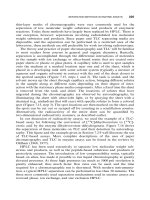
consists of a number of components, and we have opted for the following breakdown: stimulus; task; method; analysis; and measure (Figure 2.1). To illustrate our use of these terms,
consider one of the most basic experiments in the study of vision: the measurement of a
“contrast detection threshold.” A contrast detection threshold is defined as the minimum
amount of contrast necessary for a stimulus to be just detectable. Figure 2.2 illustrates the
idea for a stimulus consisting of a patch on a uniform background. The precise form of the
stimulus must, of course, be tailored to the specific question about sensory function being
asked, so we assume that the patch is the appropriate stimulus. The contrast of the patch
can be measured in terms of Weber contrast, defined as the difference between the luminance
of the patch and its background, DL, divided by the luminance of the background Lb, i.e., DL/
Lb. The contrast detection threshold is therefore the smallest value of Weber contrast needed
to detect the patch. Many procedures exist for measuring a contrast detection threshold, each
involving a different task for the observer. Before the advent of digital computers, a common
Psychophysics
experiment

Stimulus

FIGURE 2.1

Task

Method

Components of a psychophysics experiment.

Analysis

Measure

13

2.2 TASKS, METHODS, AND MEASURES

1.00

Prop. correct

0.90
0.80
0.70
0.60
0.50

CT

0.40

ΔL

Lb

0.00

0.05

0.10

0.15

Contrast

C=ΔL/Lb
FIGURE 2.2 Top left: circular test patch on a uniform background. Bottom left: luminance profile of the patch and
the definition of Weber contrast. Right: results of a standard two-interval-forced-choice (2IFC) experiment. The
various stimulus contrasts are illustrated on the abscissa. Black circles are the proportion of correct responses for
each contrast. The green curve is the best fit of a psychometric function, and the calculated contrast detection
threshold (CT) is indicated by the arrow. See text for further details. L ¼ luminance; Lb ¼ luminance of background;
DL ¼ difference in luminance between patch and background; C ¼ Weber contrast.

method was to display the stimulus on an oscilloscope and ask observers to adjust the
contrast with a dial until the stimulus was just visible. The just-visible contrast would then
be recorded as the contrast detection threshold. This method is typically termed the “method
of adjustment”, or MOA.
Nowadays the preferred approach is to present stimuli on a computer display and use a
“two-interval forced-choice,” or 2IFC, task. Using this procedure, two stimuli are presented
briefly on each trial, one of which is a blank screen, the other the test patch. The order of stimulus presentationdblank screen followed by test patch or test patch followed by blank
screendis unknown to the observer (although of course “known” to the computer) and is
typically random or quasi-random. The two stimuli are presented consecutively, and the
observer chooses the interval containing the test patch, indicating his or her choice by pressing a key. The computer keeps a record of the contrast of the patch for each trial, along with
the observer’s response, which is scored as either “correct” or “incorrect.” A given experimental session might consist of, say, 100 trials, and a number of different patch contrasts
would be presented in random order.
With the standard 2IFC task, different methods are available for selecting the contrasts presented on each trial. On the one hand, they can be preselected before the
experimentdfor example, 10 contrasts ranging from 0.01 to 0.1 at 0.01 intervals. If preselected in this way, the 10 stimuli at each contrast would be presented in random order
during the session, making 100 trials in total. This is known as the “method of constants.”
At the end of each session the computer calculates the number of correct responses for
each contrast. Typically, there would be a number of sessions and the overall proportion
correct across sessions for each patch contrast calculated, then plotted on a graph as

shown for the hypothetical data in Figure 2.2. On the other hand, one could use an “adaptive” (or “staircase”) method, in which the contrast selected on each trial is determined by


14

2. CLASSIFYING PSYCHOPHYSICAL EXPERIMENTS

the observer’s responses on previous trials. The idea behind the adaptive method is that
the computer “homes in” on the contrasts that are close to the observer’s contrast detection threshold, thus not wasting too many trials on stimuli that are either too easy or too
hard to see. Adaptive methods are the subject of Chapter 5.
The term “analysis” refers to how the data collected during an experiment are converted
into measures. For example, with the method of adjustment the observer’s settings might be
averaged to obtain the threshold. On the other hand, using the 2IFC procedure in conjunction
with the method of constants, the proportion correct data may be fitted with a function whose
shape is chosen to match the data. The fitting procedure can be used to estimate the contrast
detection threshold defined as the proportion correct, say 0.75 or 75%, as shown in Figure 2.2.
Procedures for fitting psychometric functions are discussed in Chapter 4.
To summarize, using the example of an experiment aimed at measuring a contrast detection
threshold for a patch on a uniform background, the components of a psychophysical experiment are as follows. The “stimulus” is a uniform patch of given spatial dimensions and of
various contrasts. Example “tasks” include adjustment and 2IFC. For the adjustment task, the
“method” is the method of adjustment, while for the 2IFC task one could employ the method
of constants or an adaptive method. In the case of the method of adjustment, the “analysis”
might consist of averaging the set of adjustments, whereas for the 2IFC task it might consist
of fitting a psychometric function to the proportion correct responses as a function of contrast.
For the 2IFC task in conjunction with an adaptive method, the analysis might involve averaging
contrasts, or it might involve fitting a psychometric function. The “measure” in all cases is a
contrast detection threshold, although other measures may also be extracted, such as an estimate of the variability or “error” on the threshold and the slope of the psychometric function.
The term “procedure” is used ubiquitously in psychophysics and can refer variously to the
task, method, analysis, or some combination thereof. Similarly, the term “method” has broad
usage. The other terms in our component breakdown are also often used interchangeably.

For example, the task in the contrast detection threshold experiment, whether adjustment
or 2IFC, is sometimes termed a “detection” task and sometimes a “threshold” task, while
in our taxonomy the terms “detection threshold” refer to the output measure. The lesson
here is that one needs to be flexible in the use of psychophysics terminology and not overly
constrained by any predefined scheme.
Next we consider some of the common dichotomies used to characterize different psychophysical procedures and experiments. The aim here is to introduce some common terminology, illustrate other varieties of psychophysical experiment besides contrast detection, and to
examine which, if any, of the dichotomies might be candidates for a psychophysics classification scheme.

2.3 DICHOTOMIES
2.3.1 “Class A” versus “Class B” Observations
An influential dichotomy introduced some years ago by Brindley (1970) is that between
“Class A” and “Class B” psychophysical observations. Although one rarely hears these terms
today, they are important to our understanding of the relationship between psychophysical
measurement and sensory function. Brindley used the term “observation” to describe the


15

2.3 DICHOTOMIES

Class A

Adjust

Adjust

Class B

Adjust

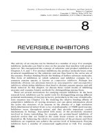
FIGURE 2.3 The Rayleigh match illustrates the difference between a Class A and Class B psychophysical
observation. For Class A, the observer adjusts both the intensity of the yellow light in the right half of the bipartite
field as well as the relative intensities of the red and green lights in the mixture in the left half of the bipartite field
until the two halves appear identical. For Class B, the observer adjusts only the relative intensities of the red and
green lights in the left half to match the hue of a yellow light in the right half that in this example is different in
brightness.

perceptual state of an observer while executing a psychophysical task. The distinction between Class A and Class B attempted to identify how directly a psychophysical observation
related to the underlying mental processes. Brindley framed the distinction in terms of a comparison of sensations: a Class A observation refers to the situation in which two physically
different stimuli are perceptually indistinguishable, whereas a Class B observation refers to
all other situations.
The best way to understand the difference between Class A and Class B is with an
example, and for this we have adopted Gescheider’s (1997) example of the Rayleigh match
(Rayleigh, 1881; Thomas and Mollon, 2004). Rayleigh matches are used to identify and study
certain types of color vision deficiency (e.g., Shevell et al., 2008), but for the present purposes
the aim of a Rayleigh match is less important than the nature of the measurement itself.
Figure 2.3 shows a bipartite circular stimulus, one half consisting of a mixture of red and
green monochromatic lights, the other half a yellow monochromatic light.1 During the
1

Because the lights are monochromatic, i.e., narrow band in wavelength, this experiment cannot be
conducted on a CRT (cathode ray tube) monitor, because CRT phosphors are relatively broadband in
wavelength. Instead an apparatus is required that can produce monochromatic lights, such as a Nagel
Anomaloscope or a Maxwellian view system.


16

2. CLASSIFYING PSYCHOPHYSICAL EXPERIMENTS

measurement procedure the observer is given free reign to adjust both the intensity of the yellow light as well as the relative intensities of the red and green lights. The task is to adjust the
lights until the two halves of the stimulus appear identical, as illustrated in the top of the
figure. In color vision, two stimuli with different spectral (i.e., wavelength) compositions
but that appear identical are termed “metamers.” According to Brindley, metameric matches
such as the Rayleigh match are Class A observations. The identification of an observation as
Class A accords with the idea that when two stimuli appear identical to the eye they elicit
identical neural responses in the brain. Since the neural responses are identical, Brindley
argues, it is relatively straightforward to map the physical characteristics of the stimuli
onto their internal neural representations.
An example of a Class B observation is shown at the bottom of Figure 2.3. This time the
observer has no control over the intensity of the yellow light, only control over the relative
intensities of the red and green lights. The task is to match the hue (or perceived chromaticity)
of the two halves of the stimulus but with the constraint that the intensity (or brightness) of the
two halves remains different. Thus, the two halves will never appear identical and therefore,
according to Brindley, neither will the neural responses they elicit. Brindley was keen to point
out that one must not conclude that Class B observations are inferior to Class A observations:
our example Class B observation is not a necessary evil due to defective equipment! On the contrary, we may wish to determine the spectral combinations that produce hue matches for stimuli that differ in brightness, precisely to understand how hue and brightness interact in the
brain. In any case, the aim here is not to judge the relative merits of Class A and Class B observations (for a discussion of this see Brindley, 1970) but rather to illustrate what the terms mean.
What other types of psychophysical experiment are Class A and Class B? According to
Brindley, experiments that measure thresholds, such as the contrast detection threshold
experiment discussed in the previous section, are Class A. This might not be intuitively
obvious, but the argument goes something like this. There are two states: stimulus present
and stimulus absent. As the stimulus contrast is decreased to a point where it is below
threshold, the observation passes from one in which the two states are discriminable to
one in which they are indiscriminable. The fact that the two states may not be discriminable
even though they are physically different (the stimulus is still present even though below
threshold) makes the observation Class A. Two other examples of Class A observations
that accord to the same criterion are shown in Figure 2.4.
Class B observations characterize many types of psychophysical procedure. Following
our example Class B observation in Figure 2.3, any experiment that involves matching

two stimuli that are perceptibly different on completion of the match is Class B. Consider,
for example, the brightness-matching experiment illustrated in Figure 2.5. The aim of this
experiment is to determine how the brightness, i.e., perceived luminance, of a test disk is
influenced by the luminance of its surround. As a rule, increasing the luminance of a surround annulus causes the disk inside to decrease in brightness, i.e., become dimmer. One
way to measure the amount of dimming is to adjust the luminance of a second, matching
disk until it appears equal in brightness to the test disk. The matching disk can be thought
of as a psychophysical “ruler.” When the matching disk is set to be equal in brightness to
the test disk, the two disks are said to be at the “point of subjective equality,” or PSE. The
luminances of the test and match disks at the PSE will not necessarily be the same; indeed it
is precisely because they are as a rule different that is of interest. The difference in


17

2.3 DICHOTOMIES

FIGURE 2.4

Two other examples of Class A observations. Top: orientation discrimination task. The observer is
required to discriminate between two gratings that differ in orientation, and a threshold orientation difference is
measured. Bottom: line bisection task. The observer is required to position the vertical red line midway along the
horizontal black line. The precision or variability in the observer’s settings is a measure of his or her line-bisection
acuity.

luminance between the test and match disks at the PSE tells us something about the effect
of context on brightness, the “context” in this example being the annulus. This type of
experiment is sometimes referred to as “asymmetric brightness matching,” because the
test and match disks are situated in different contexts (e.g., Blakeslee and McCourt,
1997; Hong and Shevell, 2004).
It might be tempting to think of an asymmetric brightness match as a Class A observation, on the grounds that it is quite different from the Class B version of the Rayleigh match

described above. In the Class B version of the Rayleigh match, the stimulus region that

(a)

Match

Test

(c)

(b)

FIGURE 2.5 Two examples of Class B observations. In (a) the goal of the experiment is to find the point of
subjective equality (PSE) in brightness between the fixed test and variable match patch as a function of the luminance (and hence contrast) of the surround annulus; (b) shows the approximate luminance profile of the stimulus;
(c) is the MullereLyer illusion. The two center lines are physically identical but appear different in length. The
experiment described in the text measures the relative lengths of the two vertical axes at which they appear equal in
length.


18

2. CLASSIFYING PSYCHOPHYSICAL EXPERIMENTS

observers match in hue is also the region that differs along the other dimensiondbrightness.
In an asymmetric brightness-matching experiment on the other hand, the stimulus region
that observers match, brightness, is not the region that differs between the test and match
stimuli - in this instance it is the annulus. However, one cannot “ignore” the annulus when
deciding whether the observation is Class A or Class B simply because it is not the part of
the stimulus to which the observation is directed. Asymmetric brightness matches are Class
B because, even when the stimuli are matched, they are recognizably different by virtue of

the fact that one stimulus has an annulus and the other does not.
Another example of a Class B observation is the MullereLyer illusion shown in
Figure 2.5(c), a geometric illusion that has received considerable attention (e.g., Morgan
et al., 1990). The lengths of the axes in the two figures are the same, yet they appear different
due to the arrangement of the fins at either end. One of the methods for measuring the size
of the illusion is to require observers to adjust the length of the axis, say of the fins-inward
stimulus, until it matches the perceived length of the axis of the other, say fins-outward stimulus. The physical difference in length at the PSE, which could be expressed as a raw, proportional, or percentage difference, is a measure of the size of the illusion. The misperception of
relative line length in the MullereLyer figures is a Class B observation, because even when
the lengths of the axes are adjusted to make them perceptually equal, the figures remain
perceptibly different as a result of their different fin arrangements.
Another example of a Class B observation is magnitude estimation. This is the procedure
whereby observers provide a numerical estimate of the perceived magnitude of a stimulus,
for example along the dimension of contrast, speed, depth, size, etc. Magnitude estimation
is Class B because our perception of the stimulus and our judgment of its magnitude utilize
different mental modalities.
An interesting case that at first defies classification into Class A or Class B is illustrated
in Figure 2.6. The observer’s task is to discriminate the mean orientation of two random
arrays of line elements, whose mean orientations are right- and left-of-vertical (e.g., Dakin,
2001). Below threshold, the mean orientations of the two arrays are indiscriminable, yet
the two arrays are still perceptibly different by virtue of their different element arrangements.
In the previously mentioned Class B examples, the “other” dimensiondbrightness in the
case of the Rayleigh match, annulus luminance in the case of the brightness-matching
experimentdwas relevant to the task. However in the mean-orientation-discrimination
experiment the “other” dimensiondelement positiondis irrelevant. Does the fact that

FIGURE 2.6

Class A or Class B? The observer’s task is to decide which of the two stimuli contains elements that
are on average left-oblique. When the difference in mean element orientation is below threshold, the stimuli are
identical in terms of their perceived mean orientation, yet are discriminable on the basis of the arrangement of their

elements.


2.3 DICHOTOMIES

19

element arrangement is irrelevant make it Class A, or does the fact that the stimuli are
discriminable below threshold on the basis of element arrangement make it Class B? Readers
can decide.
In summary, the Class A versus Class B distinction is important for understanding the
relationship between psychophysical measurement and sensory function. However, we
choose not to use this dichotomy as a basis for classifying psychophysics experiments, in
part because there are cases that seem hard to classify in terms of Class A or Class B, and
in part because other dichotomies for us better capture the critical differences between psychophysical experiments.

2.3.2 “Type 1” versus “Type 2”
An important consideration in sensory measurement concerns whether or not an observer’s responses can be designated as “correct” or “incorrect”. If they can be so designated,
the procedure is termed Type 1 and if not Type 2 (Sperling, 2008; see also Sperling et al.,
1990). The term Type 2 has sometimes been used to refer to an observer’s judgments about
their own Type 1 decisions (Galvin et al., 2003); in this case, the Type 2 judgment might be
a rating of, say, 1e5, or a binary judgment such as “confident” or “not confident,” in reference to their Type 1 decision2.
The forced-choice version of the contrast threshold experiment described earlier is a prototypical Type 1 experiment, whereas the brightness-matching and MullereLyer illusion experiments, irrespective of whether or not they employ a forced-choice procedure, are
prototypical Type 2 experiments. There is sometimes confusion, however, as to why some
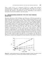
forced-choice experiments are Type 2. Consider again the MullereLyer illusion experiment.
As with the contrast detection threshold experiment, there is more than one way to measure
the size of the illusion. We have already described the adjustment procedure. Consider how
the MullereLyer might be measured using a forced-choice procedure. One method would be
to present the two fin arrangements as a forced-choice pair on each trial, with the axis of one
fixed in length and the axis of the other variable in length. Observers would be required on

each trial to indicate the fin arrangement that appeared to have the longer axis. Figure 2.7
shows hypothetical results from such an experiment. Each data point represents the proportion of times the variable-length axis is perceived as longer than the fixed-length axis, as a
function of the length of the latter. At a relative length of 1, meaning that the axes are physically the same, the observer perceives the variable axis as longer almost 100% of the time.
However, at a relative axis length of about 0.88, the observer chooses the variable axis as
longer only 50% of the time. Thus, the PSE is 0.88. However, even though the MullereLyer
experiment, like the contrast threshold experiment, can be measured using a forced-choice
procedure, there is an important difference between the two experiments. Whereas in the
contrast detection threshold experiment there is a correct and an incorrect response on every
trial, there is no correct or incorrect response for the MullereLyer trials. Whatever response
the observer makes on a MullereLyer trial, it is meaningless to score it as correct or incorrect,
at least given the goal of the experiment, which is to measure a PSE. Observers unused to
doing psychophysics often have difficulty grasping this idea and even when told repeatedly
2

Note that the dichotomy is not the same as Type I and Type II errors in statistical inference testing.


2. CLASSIFYING PSYCHOPHYSICAL EXPERIMENTS

Proportion longer responses

20

1.00

0.75

0.50

0.25

0.00
0.8

0.9

1.0

1.1

1.2

Variable/fixed length ratio
Fixed
Variable

FIGURE 2.7 Results of a hypothetical experiment aimed at measuring the size of the MullereLyer illusion using a
forced-choice procedure and the method of constant stimuli. The critical measurement is the PSE between the lengths
of the axes in the fixed test and variable comparison stimuli. The graph plots the proportion of times subjects perceive
the variable axis as “longer.” The continuous line through the data is the best-fitting logistic function (see Chapter 4).
The value of 1.0 on the abscissa indicates the point where the fixed and variable axes are physically equal in length.
The PSE is calculated as the variable axis length at which the fixed and variable axis lengths appear equal, indicated
by the vertical green arrow. The horizontal red-arrowed line is a measure of the size of the illusion.

that there are no correct and incorrect answers, insist on asking at the end of the experiment
how many trials they scored correct!
The Type 1 versus Type 2 dichotomy is not synonymous with Class A versus Class B,
though there is some overlap. For example, the Rayleigh match experiment described above
is Class A but Type 2 because no “correct” match exists. On the other hand, the two-alternative
forced-choice (2AFC) contrast threshold experiment is both Class A and Type I.

The Type 1 versus Type 2 dichotomy is an important one in psychophysics. It dictates, for
example, whether observers can be provided with feedback during an experiment, such as a
tone for an incorrect response. However, one should not conclude that Type 1 is “better” than
Type 2. The importance of Rayleigh matches (Class A but Type 2) for understanding color
deficiency is an obvious case in point.

2.3.3 “Performance” versus “Appearance”
A dichotomy related to Type 1 versus Type 2, but differing from it in important ways, is
that between “performance” and “appearance.” Performance-based tasks measure aptitude,
i.e., “how good” an observer is at a particular task. For example, suppose one measures
contrast detection thresholds for two sizes of patch, call them “small” and “big.” If thresholds for the big patch are found to be lower than those for the small patch, one can conclude
that observers are better at detecting big patches than small ones. By the same token,
if orientation discrimination thresholds are found to be lower in central than in peripheral