Performance assessment for process monitoring and fault detection methods
Bạn đang xem bản rút gọn của tài liệu. Xem và tải ngay bản đầy đủ của tài liệu tại đây (2.69 MB, 164 trang )
Kai Zhang
Performance
Assessment for Process
Monitoring and Fault
Detection Methods
Performance Assessment for Process
Monitoring and Fault Detection Methods
Kai Zhang
Performance
Assessment for Process
Monitoring and Fault
Detection Methods
Kai Zhang
Duisburg, Germany
Dissertation, Duisburg-Essen University, 2016
ISBN 978-3-658-15970-2
ISBN 978-3-658-15971-9 (eBook)
DOI 10.1007/978-3-658-15971-9
Library of Congress Control Number: 2016954529
Springer Vieweg
© Springer Fachmedien Wiesbaden GmbH 2016
This work is subject to copyright. All rights are reserved by the Publisher, whether the whole or part
of the material is concerned, specifically the rights of translation, reprinting, reuse of illustrations,
recitation, broadcasting, reproduction on microfilms or in any other physical way, and transmission
or information storage and retrieval, electronic adaptation, computer software, or by similar or
dissimilar methodology now known or hereafter developed.
The use of general descriptive names, registered names, trademarks, service marks, etc. in this
publication does not imply, even in the absence of a specific statement, that such names are exempt
from the relevant protective laws and regulations and therefore free for general use.
The publisher, the authors and the editors are safe to assume that the advice and information in this
book are believed to be true and accurate at the date of publication. Neither the publisher nor the
authors or the editors give a warranty, express or implied, with respect to the material contained
herein or for any errors or omissions that may have been made.
Printed on acid-free paper
This Springer Vieweg imprint is published by Springer Nature
The registered company is Springer Fachmedien Wiesbaden GmbH
The registered company address is: Abraham-Lincoln-Str. 46, 65189 Wiesbaden, Germany
To my parents and Sissi
Preface
With the increasing demands on product quality and process operating
safety, process monitoring and fault detection (PM-FD) has become an
important area of research in recent decades. Numerous methods were
developed in this area for different types of processes and applied to
various industrial sectors. However, there is little work focusing on comparing and assessing their performance using a unified framework, and
thus few suggestions and guidance for choosing an appropriate method
can be provided to the practitioners. Therefore, the performance assessment study for PM-FD methods has become an area of interest in both
academia and industry.
The first objective of this thesis is to assess the performance of basic
FD statistics. The commonly used two statistics, namely, T 2 and Q are
first examined. With the aid of χ2 distribution, their differences to detect
additive and multiplicative faults are revealed and compared under the
statistical framework. Due to their low detectability to multiplicative
faults, some alternative statistics are investigated.
Based on the basic FD statistics, different PM-FD methods have been
proposed to monitor the key performance indicators (KPIs) of static processes, steady-state dynamic processes and dynamic processes including
transient states. Thus, the second objective of this thesis is to assess
the three classes of KPI-based PM-FD methods. Firstly, existing static
methods are sorted into three categories based on the way to partition
the KPI-correlated part from the KPI-uncorrelated part. A new EDD
index is proposed to assess their performance to detect offsetting, drift
and multiplicative faults. Secondly, two dynamic partial least squares
(DPLS)-based methods for steady-state dynamic processes are compared,
and their performance is assessed using EDD. Furthermore, the KPIbased PM-FD methods for general dynamic processes are introduced,
some new developments are given.
Finally, to validate the theoretical developments, a case study on
the Tennessee Eastman benchmark process that can be considered as a
VIII
Preface
steady-state dynamic process is performed to assess the two DPLS-based
methods. In addition, a real large-scale hot strip rolling mill process is
applied to assess the dynamic KPI-based PM-FD methods.
This work was done while I was with the Institute for Automatic
Control and Complex Systems (AKS) at the University of DuisburgEssen, Duisburg, Germany. I would like to express my deepest gratitude
to my supervisor, Prof. Dr.-Ing. Steven X. Ding, for all the inspiration
and help he provided during the course of the last three and a half years.
I am sincerely grateful for his guidance and influence on my scientific
research work. I would also like to thank Prof. Peng for his interest in
my work. Without his valuable discussions and constructive comments,
the thesis cannot have reached the current level.
Furthermore, I would like to express my appreciation to my colleagues,
Zhiwen, Dr. Hao, Dr. Shardt, and Prof. Ge for all the impressive
discussions and cooperations on my research topic as well as for their
patience to go over the draft for this thesis. My special thanks should
once again go to Dr. Shardt, who has shared his rich and valuable
experiences on academic research and scientific writing.
In addition, I would like to thank Linlin, Changchen, Hao, Minjia,
Sihan, Dongmei, Ying, and Yong for their support during my stay in
AKS. My thanks also go to all my other AKS colleagues, Tim K., Chris,
Shane, Tim D., Sabine, Dr. K¨oppen-Seliger, Klaus, Ulrich, Dr. Qiu, Dr.
Li, and Dr. Jiang as well as my former colleagues, Prof. Lei, Prof. Shen,
Prof. Dong, and Prof. Yang for their valuable discussions and helpful
suggestions. Without them the completion of this thesis would not have
been possible.
Finally, I would like to thank the China Scholar Council (CSC) for
funding my stay in Germany.
Kai Zhang
Contents
Preface
VII
List of Figures
XIII
List of Tables
XVII
List of Notations
1 Introduction
1.1 Background and basic concepts . . . .
1.2 Motivation for the work . . . . . . . .
1.2.1 Basic FD test statistics . . . .
1.2.2 KPI-based PM-FD methods for
1.2.3 KPI-based PM-FD methods
dynamic processes . . . . . . .
1.2.4 KPI-based PM-FD methods for
1.2.5 Performance evaluation . . . .
1.3 Objectives . . . . . . . . . . . . . . . .
1.4 Outline of the thesis . . . . . . . . . .
XIX
1
. . . . . . . . . . . 1
. . . . . . . . . . . 4
. . . . . . . . . . . 4
static process . . . 6
for steady-state
. . . . . . . . . . . 8
dynamic process . 9
. . . . . . . . . . . 9
. . . . . . . . . . . 10
. . . . . . . . . . . 11
2 Basics of fault detection and performance
techniques
2.1 Technical description of static processes . . .
2.2 Technical description of dynamic processes . .
2.3 FD performance evaluation indices . . . . . .
2.3.1 FDR and FAR . . . . . . . . . . . . .
2.3.2 Expected detection delay . . . . . . .
2.4 Simulation results . . . . . . . . . . . . . . .
2.5 Conclusions . . . . . . . . . . . . . . . . . . .
evaluation
.
.
.
.
.
.
.
.
.
.
.
.
.
.
.
.
.
.
.
.
.
.
.
.
.
.
.
.
.
.
.
.
.
.
.
.
.
.
.
.
.
.
.
.
.
.
.
.
.
15
15
17
18
18
21
25
27
X
Contents
3 Common test statistics for fault detection
3.1 Background . . . . . . . . . . . . . . . . . . . . . . . .
3.2 Statistical properties of the T 2 - and Q-statistics . . . .
3.3 Detecting additive faults . . . . . . . . . . . . . . . . .
3.4 Detecting independent multiplicative faults . . . . . .
3.5 Alternative statistics for detecting multiplicative faults
3.5.1 The extension of traditional methods . . . . . .
3.5.2 Wishart distribution-based methods . . . . . .
3.5.3 Information theory-based methods . . . . . . .
3.5.4 Theoretical comparisons . . . . . . . . . . . . .
3.6 Simulation results . . . . . . . . . . . . . . . . . . . .
3.6.1 Additive faults . . . . . . . . . . . . . . . . . .
3.6.2 Multiplicative faults . . . . . . . . . . . . . . .
3.7 Conclusions . . . . . . . . . . . . . . . . . . . . . . . .
.
.
.
.
.
.
.
.
.
.
.
.
.
.
.
.
.
.
.
.
.
.
.
.
.
.
29
29
30
33
36
41
41
42
44
46
49
49
53
59
4 KPI-based PM-FD methods for static processes
4.1 Background . . . . . . . . . . . . . . . . . . . . . . .
4.2 Classification of existing approaches . . . . . . . . .
4.2.1 A direct method . . . . . . . . . . . . . . . .
4.2.2 Linear regression-based methods . . . . . . .
4.2.3 PLS-based methods . . . . . . . . . . . . . .
4.3 Theoretical comparisons . . . . . . . . . . . . . . . .
4.3.1 Interconnections among the approaches . . .
4.3.2 Geometric properties and computations . . .
4.3.3 Remarks for PM-FD . . . . . . . . . . . . .
4.4 Performance evaluation . . . . . . . . . . . . . . . .
4.4.1 A unified form of KPI-related fault detection
4.4.2 Calculation of FDR for JT 2 ,P and JQ,P . . . .
4.4.3 Simulation results . . . . . . . . . . . . . . .
4.5 Conclusions . . . . . . . . . . . . . . . . . . . . . . .
.
.
.
.
.
.
.
.
.
.
.
.
.
.
.
.
.
.
.
.
.
.
.
.
.
.
.
.
.
.
.
.
.
.
.
.
.
.
.
.
.
.
61
61
63
63
64
67
70
70
73
80
81
82
83
84
88
5 KPI-based PM-FD methods for steady-state
processes
5.1 Background . . . . . . . . . . . . . . . . . . . . .
5.2 A comparison of two DPLS models . . . . . . . .
5.2.1 Two DPLS methods . . . . . . . . . . . .
5.2.2 The NIPALS alternative . . . . . . . . . .
5.2.3 Deflations and the complete DPLS model
.
.
.
.
.
dynamic
.
.
.
.
.
.
.
.
.
.
.
.
.
.
.
.
.
.
.
.
91
92
93
93
96
98
Contents
5.3
5.4
5.5
XI
EDD-based performance evaluation . . . . . . . . . .
5.3.1 KPI-based monitoring using DPLS models . .
5.3.2 Performance evaluation with respect to EDD
Simulation results . . . . . . . . . . . . . . . . . . .
Conclusions . . . . . . . . . . . . . . . . . . . . . . .
.
.
.
.
.
.
.
.
.
.
.
.
.
.
.
100
100
101
102
107
6 KPI-based PM-FD methods for dynamic processes
6.1 Background . . . . . . . . . . . . . . . . . . . .
6.1.1 Parity-space-based fault detection . . .
6.1.2 Data-driven diagnostic observer . . . . .
6.2 KPI-based FD using DO-based method . . . .
6.3 KPI-based FD using subprocess-based method
6.4 Simulation results . . . . . . . . . . . . . . . .
6.5 Conclusions . . . . . . . . . . . . . . . . . . . .
.
.
.
.
.
.
.
.
.
.
.
.
.
.
.
.
.
.
.
.
.
.
.
.
.
.
.
.
.
.
.
.
.
.
.
.
.
.
.
.
.
.
109
109
111
112
113
115
116
118
7 Benchmark study and industrial application
7.1 Case studies on TE process . . . . . . . . . .
7.1.1 A brief introduction to TE process . .
7.1.2 Results and discussion . . . . . . . . .
7.2 Application to an industrial HSMR process .
7.2.1 An introduction to the HSMR process
7.2.2 Results and discussion . . . . . . . . .
7.3 Conclusions . . . . . . . . . . . . . . . . . . .
.
.
.
.
.
.
.
.
.
.
.
.
.
.
.
.
.
.
.
.
.
.
.
.
.
.
.
.
.
.
.
.
.
.
.
.
.
.
.
.
.
.
121
121
121
124
128
128
130
136
.
.
.
.
.
.
.
8 Conclusions and future work
137
8.1 Conclusions . . . . . . . . . . . . . . . . . . . . . . . . . . 137
8.2 Future work . . . . . . . . . . . . . . . . . . . . . . . . . . 139
Bibliography
141
List of Figures
1.1
1.2
1.3
1.4
Schematic description of an industrial process
Schematic description of PM-FD methods . .
Basics of statistical fault detection methods .
Structure of the thesis . . . . . . . . . . . . .
2.1
2.2
2.3
Demonstration of additive and multiplicative faults . . . .
Demonstration of false alarm rate and fault detection rate
Schematic description of detection delay using FAR and
FDR . . . . . . . . . . . . . . . . . . . . . . . . . . . . . .
An example with FDR for a drift fault . . . . . . . . . . .
EDD performance for constant additive faults . . . . . . .
EDD performance for drift faults . . . . . . . . . . . . . .
EDD performance for constant multiplicative faults . . . .
2.4
2.5
2.6
2.7
3.1
3.2
3.3
3.4
3.5
3.6
.
.
.
.
.
.
.
.
.
.
.
.
.
.
.
.
.
.
.
.
.
.
.
.
. 2
. 3
. 5
. 13
Demonstration of JT 2 for detecting additive faults . . . .
Demonstration of JT 2 for detecting multiplicative faults .
Comparison of FDR for additive and multiplicative faults
Different thresholds for JT 2 and JQ . . . . . . . . . . . . .
Demonstration of JT 2 and JQ for detecting additive faults
Schematic description of JT 2 and JQ for detecting
multiplicative faults . . . . . . . . . . . . . . . . . . . . .
3.7 Performance of ϑ with different gf and hf , m = 10, n = 10
3.8 Performance of ϑ with different n, m = 10 . . . . . . . . .
3.9 Performance of JT 2 , JTn2 , JQ and JQn for Scenario 1 . . .
3.10 Performance of Jγ , JT and JD for Scenario 1 . . . . . . .
3.11 Performance of JL for Scenario 1 . . . . . . . . . . . . . .
3.12 Performance of different statistics for Scenario 2 . . . . .
4.1
4.2
19
20
23
24
26
26
27
34
39
40
50
52
54
55
55
57
57
58
58
Demonstration of the projections of the direct method . . 77
Demonstration of the projections of LS and PCR . . . . . 78
XIV
4.3
4.4
4.5
5.1
5.2
List of Figures
Demonstration of the projection relationship
PLS and T-PLS . . . . . . . . . . . . . . . . . .
Demonstration of the projection relationship
PLS and C-PLS . . . . . . . . . . . . . . . . . .
Flops costed by the examined methods . . . . .
between
. . . . . . 78
between
. . . . . . 79
. . . . . . 80
103
5.4
5.5
5.6
Cross-validation results in the numerical example . . . . .
The mixture of AIC and cross-validation result in the
numerical example . . . . . . . . . . . . . . . . . . . . . .
Comparison of the original method to the alterative
NIAPLS method . . . . . . . . . . . . . . . . . . . . . . .
AIC results of the VAR model in the numerical example .
Residuals obtained by performing VAR model on t. . . . .
Comparison of EDD in the numerical example . . . . . . .
6.1
6.2
6.3
6.4
6.5
Detection performance for Scenario 1 . . . . .
Profile of variables in Scenario 2 . . . . . . .
Fault detection performance for fault Scenario
Profile of variables in Scenario 3 . . . . . . .
Fault detection performance for fault Scenario
.
.
.
.
.
117
118
118
119
119
7.1
7.2
Schematic description of the TE process . . . . . . . . . .
Detection performance for fault-free case using two DPLS
methods . . . . . . . . . . . . . . . . . . . . . . . . . . . .
Detection of fault 1 using two DPLS methods . . . . . . .
Probability distribution of DD for fault 7 using two DPLS
methods . . . . . . . . . . . . . . . . . . . . . . . . . . . .
Probability distribution of DD for fault 4 using two DPLS
methods. . . . . . . . . . . . . . . . . . . . . . . . . . . .
Schematic description of a large-scale FMP . . . . . . . .
Schematic description of the stand in FMP . . . . . . . .
Normal distribution plot of residual signals using DObased method . . . . . . . . . . . . . . . . . . . . . . . . .
Normal distribution plot of residual signals for subprocess
1 and 2 . . . . . . . . . . . . . . . . . . . . . . . . . . . .
Monitoring result for Scenario 1 . . . . . . . . . . . . . . .
Monitoring result for Scenario 2 . . . . . . . . . . . . . . .
Monitoring result for Scenario 2 using DO-based method .
Monitoring result for Scenario 3 . . . . . . . . . . . . . . .
122
5.3
7.3
7.4
7.5
7.6
7.7
7.8
7.9
7.10
7.11
7.12
7.13
. .
. .
2.
. .
3.
.
.
.
.
.
.
.
.
.
.
.
.
.
.
.
.
.
.
.
.
104
104
105
105
106
125
126
127
127
129
130
131
132
133
133
134
134
List of Figures
XV
7.14 Monitoring result for Scenario 3 using DO-based method . 135
7.15 Monitoring result for Scenario 4 . . . . . . . . . . . . . . . 135
7.16 Monitoring result for Scenario 4 using DO-based method . 136
List of Tables
3.1
3.2
4.1
4.2
4.3
4.4
4.5
4.6
4.7
5.1
5.2
5.3
5.4
5.5
7.1
7.2
Comparison of different test statistics for multiplicative
faults . . . . . . . . . . . . . . . . . . . . . . . . . . . . . 46
FDR for different additive faults (JT 2 /JQ ) . . . . . . . . . 52
Summary of projectors . . . . . . . . . . . . . . . . . . . .
Information about KPI-correlated subspaces . . . . . . . .
Summary of the computational complexity and parameter
EDD for different KPI-related faults for the numerical
example . . . . . . . . . . . . . . . . . . . . . . . . . . . .
EDD for KPI-unrelated faults in numerical example . . .
EDD for different multiplicative faults . . . . . . . . . . .
EDD for different drift faults . . . . . . . . . . . . . . . .
76
77
80
Original algorithm for the DDPLS method . . . .
Original algorithm for the IDPLS method . . . .
NIPALS algorithm for the DDPLS method . . .
NIPALS algorithm for the IDPLS method . . . .
Comparison of the average EDD given by two
methods . . . . . . . . . . . . . . . . . . . . . . .
94
96
96
98
. . . . .
. . . . .
. . . . .
. . . . .
DPLS
. . . . .
85
86
87
88
106
Process and manipulated variables of TE process . . . . . 123
EDD of two DPLS methods for additive faults in TE
process . . . . . . . . . . . . . . . . . . . . . . . . . . . . . 126
Abbreviations and notations
Abbreviations
Abbreviation
AIC
ARMA
CCA
CDF
C-PLS
DD
DDPLS
DO
DPLS
EDD
FAR
FD
FDR
FIR
FMP
HSMR
IDPLS
KPI
LS
LTI
MSPM
NIPALS
PCA
PCR
PLS
PM
PM-FD
PRESS
Expansion
Akaike Information Criterion
Auto-Regressive Moving Average
Canonical Correlation Analysis
Cumulative Distribution Function
Concurrent Partial Least Squares
Detection Delay
Direct Dynamic Partial Least Squares
Diagnostic Observer
Dynamic Partial Least Squares
Expected Detection Delay
False Alarm Rate
Fault Detection
Fault Detection Rate
Finite Impulse Response
Finishing Mill Process
Hot Strip Mill Rolling
Indirect Dynamic Partial Least Squares
Key Performance Indicator
Least Squares
Linear Time-Invariant
Multivariate Statistical Process Monitoring
Nonlinear Iterative PArtial Least Squares
Principal Component Analysis
Principal Component Regression
Probability Distribution Function
Partial Least Squares
Process Monitoring
Process Monitoring and Fault Detection
Predicted REsidual Sum of Squares
List of Notations
XX
PS
SVD
TE
T-PLS
VAR
Parity Space
Singular Vector Decomposition
Tennessee Eastman
Total Partial Least Squares
Vector Auto-Regression
Mathematical notations
Notation
∀
∼
≈
≫
→
Rm
Rm×n
Im
|| · ||E
|| · ||F
|| · ||2
|·|
c
y
y(i)
yi
Y
ˆ
y
˜
y
YT
Y−1
Y†
Y⊥
f
f
Ξ
λ
σ
Description
For all
Follow
Approximately equal
Defined as
Much larger than
From...to
Set of m-dimensional real vectors
Set of m × n-dimensional real matrices
m-dimensional identify matrix
Euclidean norm of a vector
Frobenius norm of a matrix
2-norm of a matrix
Determinant of a matrix or absolute value
A real constant
A vector
The ith element of y or the ith sample of y
ith iteration of y
A matrix
Estimate of y or KPI-related part in y
Residual of y, or KPI-unrelated part in y
Transpose of Y
Inverse of a square matrix Y
Pseduoinverse of Y
Orthogonal complement of Y
Fault vector
Fault magnitude
Fault direction
Eigenvalue
Singular value or standard derivation
List of Notations
tr(Y)
diag(y)
rank(Y)
dim{·}
span{y}
⊕
⊗
∝
E (·)
Var (·)
Cov (·)
prob (x)
Nm (µ, Σ)
J
Jth
χ2m
χ2m (δ)
F (a, b)
α
χ2m,α
Fα (a, b)
Wm (Σ, n)
e, exp(·)
XXI
Trace of Y
A diagonal matrix with non-zeros elements y
Rank of matrix Y
Dimension of a space
Space spanned by y
Direct sum of two vector-spanned spaces
Kronecker product
Proportional
Mean value/vector
Variance value/vector
Covariance matrix
Probability of x
m-dimensioned Normal/Gaussian distribution
with mean µ and covariance matrix Σ
Test statistic
Threshold
Chi-squared distribution with m degrees
of freedom
Noncentral χ2 distribution with m degrees
of freedom and noncentrality parameter δ
F distribution with a and b degrees of freedom
Significance level
Confidence value corresponding to α
Confidence value corresponding to α
Wishart distribution with n degrees of freedom
based on m-dimensional covariance matrix Σ
Base of natural logarithm, natural exponential
function
1 Introduction
1.1 Background and basic concepts
Consider a typical industrial process as shown in Figure 1.1. Control
signals sent from the controller are feeded into actuators, where the
process input signals are generated. The process is driven by the input
signals to achieve the desired output behavior. Finally, sensors convert
the output variables as measurement variables, which provide essential
information for implementing closed-loop control. It is common for a
real process that all these components are subject to disturbances in a
stochastic manner. As a result, the input and output signals as well as
the measurements are corrupted with noise. An example to this problem
is the white noise in measurements, which is due to the accuracy of the
sensor and noisy ambient. In reality, such processes are threaten by
various faults that may occur in all components. They can not only break
the control loop at the process level, but also cause unexpected changes
in the plant level. To achieve optimal process operation, these faults
should be readily and accurately detected. This, thus, motivates and
drives the development of fault detection (FD) methods in both theory
and practice. Conceptually, these methods deal with the following task
[1–5]:
Fault detection: detection of the abnormal events in the functional
units of the process, which can lead to undesired or unacceptable
behavior of the whole plant.
It is noted that FD methods are commonly performed at the process level,
which means there should be sufficient process knowledge including at
least process input and output information. As well known, large-scale
processes are ubiquitous features of many chemical, steelmaking and
papermaking plants. Such large-scale processes consist of great number
of interacting subprocesses which increase the overall control complexity.
© Springer Fachmedien Wiesbaden GmbH 2016
K. Zhang, Performance Assessment for Process Monitoring and
Fault Detection Methods, DOI 10.1007/978-3-658-15971-9_1
2
1 Introduction
Faults
Disturbances
Control
signals
Actuators
Input
signals
Output
signals
Process
Measurements
Sensors
Figure 1.1: Schematic description of an industrial process
Due to increasing demands for quality, a greater emphasis on improving
operating performance of these large-scale processes can be observed.
This results in strong needs to monitor the process operation at the
plant level. Consequently, process monitoring (PM) methods have been
extensively reported in the last two decades and widely applied in various
industrial plant, such as chemical industry, semiconductor manufacture,
steel industry etc. A technical description of process monitoring, as given
in [14, 18, 77, 85, 111] is
Process monitoring: often referred as statistical process monitoring,
generally defined as the use of statistical methods to monitor the
operation of the process to improve process quality and productivity
Aiming at PM, two groups of methods are generally used. The first
group check the entire process measurements for the purpose of monitoring the performance of the whole plant. Another group pays the
attention to the performance of the most important variables. These
variables are not always easily measured but can directly indicate the
plant operating performance, which has recently been adopted as key
performance indicators (KPIs) to analyse the process performance [6, 8].
Hao et al. [7], showed that industrial KPIs can be classified into three
groups:
• engineering KPIs that refer to the technical performance of the
plant, for example, product quality;
• maintenance KPIs that refer to the operating rate and hence maintenance time and costs;
• economic KPIs that refer to business profit, for example, the overall
energy consumption or the productivity of a plant.
1.1 Background and basic concepts
3
PM-FD methods for control loop
performance (process-level)
Key Performance
Indicators (KPIs)
PM-FD methods
for KPI performance
(plant-level)
Process
Actuators
Controllers
Sensors
PM-FD methods for process operating
performance (plant-level)
Figure 1.2: Schematic description of PM-FD methods
It has been shown that KPIs are closely related to the measurable process variables, but difficult to be directly measured [8, 28], for example,
the concentration in a chemical process or the thickness of a steel roll
between two stands in the steel mill process. KPI-based PM methods are
primarily developed by applying the online readily measurable variables
to track the behavior of KPIs. This kind of approaches have been shown
being powerful and effective in detecting process faults that negatively
influence KPIs and so enhancing the product quality. It can likewise
be seen that KPI-based PM methods are performed at the plant level.
Note that although FD and PM methods occur in different levels, from
the statistical perspective, there are mixture use of them in literature
[40]. It is common that reporting the process as normal or not can also
be regarded as determining wether a fault occurred or not in the FD
method. In this thesis, in order to avoid the terminological misleading,
process monitoring and fault detection (PM-FD) will be adopted to account for plant-level methods. The overall PM-FD issues addressed in
industrial plants are structured in Figure 1.2 [13]. Due to the increase in
demanding high quality products and high-efficiency performance, this
thesis focuses on the KPI-based PM-FD methods.
4
1 Introduction
1.2 Motivation for the work
1.2.1 Basic FD test statistics
Process maintenance and management require detailed process operating
information to determine not only whether the process is operating normally, but also to determine the potential causes for any observed problems [118]. In modern industrial plants, multidimensional, correlated
process data are ubiquitous. The challenging issue is how to determine if
the data are informative enough to monitor the process and which methods can be used to achieve this. One approach to this problem is through
the PM-FD [36] that seeks to examine the information provided by routine operating data to determine the existence of problems and their
probable root causes. Early work in this field was performed by Walter
Shewhart in the early 1920s [53, 107], who developed Shewhart control
charts that allows easily tracking of the reliability of telephony transmission systems. Afterwards, this approach has been widely adopted in
other technically and physical processes, where a normal distribution is
typically assumed. Shewhart charts are easy to create, but are limited to
univariate monitoring which does not take into consideration any dependencies between the monitored variables [53]. Driven by the demands of
safety and regulation in industrial plants, countless KPI-based PM-FD
approaches have been developed for easy tracking of the KPI variable
[13]. Due to the stochastic disturbances, as shown in Figure 1.1, using
solely the mean of process variables as a sufficient descriptor is dubious.
In fact, it would be better to consider the probability distribution of
the process variable. The most common solution to this issue is using
multivariate statistical techniques, where process variables are assumed
to follow multivariate normally distribution. In this framework, multivariate detection statistics are then developed which can simultaneously
monitor an ensemble of variables to determine whether the process is behaving properly. For example, a process with two Gaussian distributed
process variable is shown in Figure 1.3. A multivariate statistics-based
approach seeks to convert the two variables to be an indicator variable
that can follow a specific distribution (e.g., χ2 -distribution in Figure 1.3)
[130], so that tracking the behavior of the indicator variable would be
equivalent to tracking the original multiple variables. Such methods, on
the one hand, can avoid separately monitoring the two variables. On the
other hand, the dependency between them is taken into account which
1.2 Motivation for the work
5
The first process variable
5
0
-5
0
50
100
150
200
250
300
350
400
450
500
400
450
500
The second process varaible
4
2
0
-2
0
50
100
150
200
250
300
350
Samples
Indicator variable
12
0.5
0.45
10
0.4
0.35
Probability
8
6
4
0.3
0.25
0.2
0.15
0.1
2
0.05
0
0
0
50
100
150
200
250
Samples
300
350
400
450
500
0
1
2
3
4
5
6
7
8
9
10
Value of indicator variable
Figure 1.3: Basics of statistical fault detection methods
can improve the FD performance. The transformations/conversions that
always refer to the fault detection statistics (J) serve as the core of statistical PM-FD methods. Using some specific probability distributions,
a upper threshold Jth or two thresholds: the upper one, Jth,1 and lower
one, Jth,2 , are determined. A faulty or normal operating status can then
be determined by comparing J with Jth . The most widely used detection
statistics are T 2 - and Q-statistics [2, 48, 52, 54, 69, 73].
In PM-FD field, two types of faults are commonly considered: additive
faults, which impact the mean of the variable, and multiplicative faults,
which lead to variation in the variance and covariance of the variables
[42]. Although additive faults are most commonly assumed in the literature [9, 64], multiplicative faults can also degrade the process efficiency,
and impact the safety of the overall system. In previous research, the
suitability of T 2 and Q-statistics for detecting these two types of faults was often checked by approximating the fault detection rate (FDR)
index using a numerical approximation-based method [71]. However, a
theoretical approach to the problem is more required. To establish a
clear mathematical foundation for them can lead to their developments
and support the implementations in PM-FD methods.
6
1 Introduction
Unlike mean change faults, the multiplicative fault will cause changes
in elements of the covariance matrix. To detect the process change that
could impact the covariance structure, some other efficient statistics are
available. They can be developed based on an individual sample or a
sequential of process data covered by a moving window-based approach
which includes enough faulty information. Although many methods have
been proposed to detect this type of faults [42, 63–65, 67, 100, 102, 103],
and some useful tools in communication field such as entropy [107], mutual information [108] and Kullback-Leibler divergence [67, 68, 70, 103, 132]
have been reported to be efficient in dealing with this type of change in
signals, there is little work focusing on reviewing them as well as comparing them by means of revealing their potential interconnections.
1.2.2 KPI-based PM-FD methods for static process
In static processes, it is assumed that process variables have no autocorrelations, and current KPI measurements can only be influenced by
current process measurements. At the same time as the development of
fault detection statistics had occurred, work in chemometrics led to the
development of new data analysis methods, for example, principal component analysis (PCA) and partial least squares (PLS) [78, 79, 92, 121],
which led to increased process efficiencies [25, 30, 35, 36, 122, 125, 127]
and understanding [36, 39, 50, 80, 123]. Finally, in the early 1990s, the
PLS and PCA methods were combined with T 2 - and Q-statistics leading
to the development of a new field of PM-FD approaches for static processes [19–21]. The pioneer work was started by MacGregor [15–17], and
successively developed by the work of Qin et al. [13, 14], and Venkatasubramanian et al. [115–117]. These methods are primarily called multivariate statistics process monitoring (MSPM)-based or data-driven methods
[13], and can be well structured in the process control framework as
shown in Figure 1.2 as plant-level methods. It is shown that they take
all the information about the process components (actuators, sensors,
controllers, and KPI) in a process control loop into consideration. Thus,
they can address different types of process faults. The general procedure
is to develop analytical models of normal and faulty operating conditions,
onto which the current process data can be projected to give a measure
of current process performance [118]. The key difference between the
PCA- and PLS-based methods is the way of using the available data s-
1.2 Motivation for the work
7
pace. As shown in Figure 1.2, PCA-based methods monitor the complete
data space [11, 14], while PLS-based methods monitor solely a subspace
of the complete data space, commonly referred to as the KPI-correlated
subspace [2]. Due to the lack of first principles models, MSPM has been
quickly adopted by chemical engineers [24, 25, 29, 37]. As well, such
methods have been applied to such areas as semiconductor, polymers,
iron, and steel processes [10, 26]. Although many different approaches
to PCA and PLS have been reported in the literature, few of them follow a unified framework that explicitly utilizes the T 2 - and Q-statistics
[27, 40, 71].
Over the past few years, great effort has been made on the modification of PLS aiming at improving the KPI-based PM-FD performance.
Representative approaches are total PLS (T-PLS) [37] and concurrent
PLS (C-PLS) [24]. Despite showing strong applicability in MSPM area,
PLS was originally proposed as an alterative of least squares (LS) in linear regression field [38, 39]. The typical linear regression-based methods
are studied by Ding et al. [6] and Yin et al. [40]. Note that a simple
method directly decomposing the cross-covariance between process and
KPI variables can also solve this problem, while it has not drawn much
attention. Finally, it is noted that even though these methods are reported to be practical in industrial application, few of them have been
theoretically assessed to determine their performance [27, 40, 41].
In many industrial applications, MSPM methods are used to detect
faults, of which the most common application is to detect additive faults,
that is, those which change the mean value of the process. The application and assessment of these methods to detect multiplicative faults,
which impact the variance or covariance parameters of process variables
are rarely considered. In [9], Hao et al. have shown, by comparing the
original and current formulae for the T 2 -statistic, that MSPM methods
could be applied to multiplicative faults. However, greater details, specially from a statistical viewpoint, are required before such methods can
be applied to detect multiplicative faults. In addition to this approach,
many other methods have been proposed for detecting multiplicative
faults [64, 66, 67]. Although many improvements on above-mentioned
methods in the literature have been reported [24, 30, 37, 80], these methods cannot well address cases that KPI variables are dynamically related
to process variables.
8
1 Introduction
1.2.3 KPI-based PM-FD methods for steady-state
dynamic processes
For dynamic processes operating in steady state [82], to address the dynamic issue, dynamic PLS (DPLS) models were proposed [12, 83, 84, 88–
90, 126], and quickly adopted both in control engineering and PM-FD
fields [34, 83, 87, 88, 91, 94]. While PLS models developed using data
independent of time, DPLS models are built based on data at current
and past time, and attempt to interpret the current KPI using sufficient
past process information [12]. Although different DPLS methods were
proposed, those that use the augmented process data to model KPI have
major focuses [12, 86, 91]. They follow the similar procedure with PLS
models, which allows an easy understanding and implementation. The
core idea is to extract the useful information from the current and past
process data, and combine them to predict the current KPI. Based on
how they determine the weighting vector to extract the KPI-relevant information, two DPLS methods are obtained, the direct DPLS (DDPLS)
method, which uses different weighting vectors [88], and the indirect DPLS (IDPLS) method, which uses the constant weighting vector [12].
Although the two DPLS methods are extensively applied, to date there
has been no detailed study on them in terms of computation, convergence characteristic, and potential relationships. Furthermore, since the
development of the nonlinear iterative partial least squares (NIPALS)
method for PLS models [21, 89, 92], extending it to the above two DPLS
methods would be useful, because it would avoid an eigenvalue decomposition performed on a high dimensional matrix. As well, it would make
it straightforward to identify and understand the difference between the
two DPLS methods.
Application of DPLS to KPI-relevant PM-FD was motivated by the
successful application of PLS-based methods [88], where it assumes that
the scores of DPLS that represent the KPI-relevant information in process data are time independent. However, this is not always the case in
actual circumstance. Recently, Li et al. proposed an approach that fits
a vector autoregression (VAR) model to the resulting scores [12]. The
VAR model is then adopted to obtain the residual vector for KPI-based
PM-FD. This method was shown to be effective and extended to dynamic
PCA-based methods [93]. To assess the performance of DPLS methods
for PM-FD, this approach will be incorporated into DPLS methods.