Simple mathematical models of gene regulatory dynamics
Bạn đang xem bản rút gọn của tài liệu. Xem và tải ngay bản đầy đủ của tài liệu tại đây (2.38 MB, 128 trang )
Lecture Notes on Mathematical Modelling
in the Life Sciences
Michael C. Mackey
Moisés Santillán
Marta Tyran-Kamińska
Eduardo S. Zeron
Simple
Mathematical Models
of Gene Regulatory
Dynamics
Lecture Notes on Mathematical Modelling
in the Life Sciences
Editors-in-Chief:
Michael C. Mackey
Angela Stevens
Series editors
Martin Burger
Maurice Chacron
Odo Diekmann
Anita Layton
Jinzhi Lei
Mark Lewis
Lakshminarayanan Mahadevan
Philip Maini
Masayasu Mimura
Claudia Neuhauser
Hans G. Othmer
Mark Peletier
Alan S Perelson
Charles S. Peskin
Luigi Preziosi
Jonathan Rubin
Moisés Santillán
Christoph Schütte
The rapid pace and development of the research in mathematics, biology and
medicine has opened a niche for a new type of publication - short, up-to-date,
readable lecture notes covering the breadth of mathematical modelling, analysis
and computation in the life-sciences, at a high level, in both printed and electronic
versions. The volumes in this series are written in a style accessible to researchers,
professionals and graduate students in the mathematical and biological sciences.
They can serve as an introduction to recent and emerging subject areas and/or as an
advanced teaching aid at colleges, institutes and universities. Besides monographs,
we envision that this series will also provide an outlet for material less formally
presented and more anticipatory of future needs, yet of immediate interest because
of the novelty of its treatment of an application, or of the mathematics being
developed in the context of exciting applications. It is important to note that
the LMML focuses on books by one or more authors, not on edited volumes.
The topics in LMML range from the molecular through the organismal to the
population level, e.g. genes and proteins, evolution, cell biology, developmental
biology, neuroscience, organ, tissue and whole body science, immunology and
disease, bioengineering and biofluids, population biology and systems biology.
Mathematical methods include dynamical systems, ergodic theory, partial differential equations, calculus of variations, numerical analysis and scientific computing,
differential geometry, topology, optimal control, probability, stochastics, statistical
mechanics, combinatorics, algebra, number theory, etc., which contribute to a
deeper understanding of biomedical problems.
More information about this series at />
Michael C. Mackey • Moisés Santillán •
Marta Tyran-Kami´nska • Eduardo S. Zeron
Simple Mathematical Models
of Gene Regulatory
Dynamics
123
Michael C. Mackey
Department of Physiology
McGill University
Montreal, QC
Canada
Moisés Santillán
Unidad Monterrey
Cinvestav del IPN
Apodaca, NL
Mexico
Marta Tyran-Kami´nska
Institute of Mathematics
University of Silesia
Katowice
Poland
Eduardo S. Zeron
Departamento de Matemáticas
Cinvestav del IPN
Ciudad de México
Mexico
ISSN 2193-4789
ISSN 2193-4797 (electronic)
Lecture Notes on Mathematical Modelling in the Life Sciences
ISBN 978-3-319-45317-0
ISBN 978-3-319-45318-7 (eBook)
DOI 10.1007/978-3-319-45318-7
Library of Congress Control Number: 2016956565
© Springer International Publishing Switzerland 2016
This work is subject to copyright. All rights are reserved by the Publisher, whether the whole or part of
the material is concerned, specifically the rights of translation, reprinting, reuse of illustrations, recitation,
broadcasting, reproduction on microfilms or in any other physical way, and transmission or information
storage and retrieval, electronic adaptation, computer software, or by similar or dissimilar methodology
now known or hereafter developed.
The use of general descriptive names, registered names, trademarks, service marks, etc. in this publication
does not imply, even in the absence of a specific statement, that such names are exempt from the relevant
protective laws and regulations and therefore free for general use.
The publisher, the authors and the editors are safe to assume that the advice and information in this book
are believed to be true and accurate at the date of publication. Neither the publisher nor the authors or
the editors give a warranty, express or implied, with respect to the material contained herein or for any
errors or omissions that may have been made.
Printed on acid-free paper
This Springer imprint is published by Springer Nature
The registered company is Springer International Publishing AG Switzerland
The registered company address is: Gewerbestrasse 11, 6330 Cham, Switzerland
To students everywhere: past, present,
and future.
Preface
We survey work that has been carried out in the attempts of biomathematicians
to understand the dynamic behavior of simple bacterial operons starting with the
initial work of the 1960s. We concentrate on the simplest of situations, discussing
both repressible and inducible systems as well as the bistable switch and then
turning to a discussion of the role of both extrinsic noise and the so-called intrinsic
noise in the form of translational and/or transcriptional bursting. We conclude with
a consideration of the messier concrete examples of the lactose and tryptophan
operons and the lysis-lysogeny switch of phage . This survey has grown out of
our work over the past 20 years and is an enlarged version of our review paper
(Mackey et al. 2015).
Montreal, QC, Canada
Apodaca, NL, Mexico
Katowice, Poland
Ciudad de México, Mexico
June 2016
Michael C. Mackey
Moisés Santillán
Marta Tyran-Kami´nska
Eduardo S. Zeron
vii
Acknowledgments
We have benefited from the comments, suggestions, and criticisms of many
colleagues over the years (you will know who you are) and from the institutional
support of our home universities as well as the University of Oxford, the University
of Bremen, Bergischen Universität Wuppertal, and the International Centre for
Theoretical Physics. MCM is especially grateful to a comment from Dr. Jérôme
Losson many years ago that directed attention to these fascinating problems.
This work was supported by the Natural Sciences and Engineering Research
Council (NSERC) of Canada, the Polish NCN grant no. 2014/13/B/ST1/00224, and
the Consejo Nacional de Ciencia y Tecnología (Conacyt) in México.
ix
Contents
Part I
Deterministic Modeling Techniques
1 Generic Deterministic Models of Prokaryotic Gene Regulation .. . . . . . .
1.1 Inducible Regulation .. . . . . . . . . . . . . . . . . . . . . . . . . . . . . . .. . . . . . . . . . . . . . . . . . . .
1.2 Repressible Regulation . . . . . . . . . . . . . . . . . . . . . . . . . . . . .. . . . . . . . . . . . . . . . . . . .
3
3
5
2 General Dynamic Considerations . . . . . . . . . . . . . . . . . . . . .. . . . . . . . . . . . . . . . . . . .
2.1 Operon Dynamics .. . . . . . . . . . . . . . . . . . . . . . . . . . . . . . . . . .. . . . . . . . . . . . . . . . . . . .
2.1.1 No Control . . . . . . . . . . . . . . . . . . . . . . . . . . . . . . . . . .. . . . . . . . . . . . . . . . . . . .
2.1.2 Inducible Regulation.. . . . . . . . . . . . . . . . . . . . . . .. . . . . . . . . . . . . . . . . . . .
2.1.3 Repressible Regulation . . . . . . . . . . . . . . . . . . . . .. . . . . . . . . . . . . . . . . . . .
2.1.4 Bistable Switches . . . . . . . . . . . . . . . . . . . . . . . . . . .. . . . . . . . . . . . . . . . . . . .
2.2 The Appearance of Cell Growth Effects and Delays Due
to Transcription and Translation.. . . . . . . . . . . . . . . . . . .. . . . . . . . . . . . . . . . . . . .
2.3 Fast and Slow Variables.. . . . . . . . . . . . . . . . . . . . . . . . . . . .. . . . . . . . . . . . . . . . . . . .
7
7
9
9
13
13
Part II
23
26
Dealing with Noise
3 Master Equation Modeling Approaches . . . . . . . . . . . . . .. . . . . . . . . . . . . . . . . . . .
3.1 The Chemical Master Equation . . . . . . . . . . . . . . . . . . . .. . . . . . . . . . . . . . . . . . . .
3.2 Relation to Deterministic Models . . . . . . . . . . . . . . . . . .. . . . . . . . . . . . . . . . . . . .
3.2.1 The Chemical Langevin Equation . . . . . . . . .. . . . . . . . . . . . . . . . . . . .
3.3 Stability of the Chemical Master Equation . . . . . . . .. . . . . . . . . . . . . . . . . . . .
3.3.1 Algorithms to Find Steady State Density Functions . . . . . . . . . .
3.4 Application to a Simple Repressible Operon . . . . . .. . . . . . . . . . . . . . . . . . . .
31
32
34
36
37
40
43
4 Noise Effects in Gene Regulation: Intrinsic Versus Extrinsic . . . . . . . . . .
4.1 Dynamics with Bursting . . . . . . . . . . . . . . . . . . . . . . . . . . . .. . . . . . . . . . . . . . . . . . . .
4.1.1 Generalities . . . . . . . . . . . . . . . . . . . . . . . . . . . . . . . . .. . . . . . . . . . . . . . . . . . . .
4.1.2 Distributions in the Presence of Bursting
for Inducible and Repressible Systems . . . .. . . . . . . . . . . . . . . . . . . .
4.1.3 Bursting in a Switch . . . . . . . . . . . . . . . . . . . . . . . .. . . . . . . . . . . . . . . . . . . .
49
50
50
52
57
xi
xii
Contents
4.1.4 Recovering the Deterministic Case . . . . . . . .. . . . . . . . . . . . . . . . . . . .
4.1.5 A Discrete Space Bursting Model . . . . . . . . .. . . . . . . . . . . . . . . . . . . .
4.2 Gaussian Distributed Noise in the Molecular Degradation Rate. . . . . .
4.3 Two Dominant Slow Genes with Bursting . . . . . . . . .. . . . . . . . . . . . . . . . . . . .
Part III
61
62
64
66
Specific Examples
5 The Lactose Operon .. . . . . . . . . . . . . . . . . . . . . . . . . . . . . . . . . . . .. . . . . . . . . . . . . . . . . . . .
5.1 The Lactose Operon Regulatory Pathway . . . . . . . . .. . . . . . . . . . . . . . . . . . . .
5.2 Mathematical Modeling of the Lactose Operon . . .. . . . . . . . . . . . . . . . . . . .
5.3 Quantitative Studies of the Lactose Operon Dynamics . . . . . . . . . . . . . . .
73
73
77
83
6 The Tryptophan Operon .. . . . . . . . . . . . . . . . . . . . . . . . . . . . . . .. . . . . . . . . . . . . . . . . . . .
6.1 The Tryptophan Operon in E. coli.. . . . . . . . . . . . . . . . .. . . . . . . . . . . . . . . . . . . .
6.2 Mathematical Modeling of the trp Operon . . . . . . . .. . . . . . . . . . . . . . . . . . . .
6.3 Quantitative Studies of the trp Operon .. . . . . . . . . . . .. . . . . . . . . . . . . . . . . . . .
87
87
89
92
7 The Lysis-Lysogeny Switch . . . . . . . . . . . . . . . . . . . . . . . . . . . . .. . . . . . . . . . . . . . . . . . . .
7.1 Phage Biology . . . . . . . . . . . . . . . . . . . . . . . . . . . . . . . . . . . .. . . . . . . . . . . . . . . . . . . .
7.2 The Lysis-Lysogeny Switch . . . . . . . . . . . . . . . . . . . . . . . .. . . . . . . . . . . . . . . . . . . .
7.3 Mathematical Modeling of the Phage Switch . . .. . . . . . . . . . . . . . . . . . . .
7.4 Brief Review of Quantitative Studies on the Phage Switch .. . . . . . . .
7.5 Closing Remarks .. . . . . . . . . . . . . . . . . . . . . . . . . . . . . . . . . . .. . . . . . . . . . . . . . . . . . . .
99
102
104
107
112
114
References .. .. . . . . . . . . . . . . . . . . . . . . . . . . . . . . . . . . . . . . . . . . . . . . . . . . .. . . . . . . . . . . . . . . . . . . . 115
Index . . . . . . . . .. . . . . . . . . . . . . . . . . . . . . . . . . . . . . . . . . . . . . . . . . . . . . . . . . .. . . . . . . . . . . . . . . . . . . . 123
Introduction
The operon concept for the regulation of bacterial genes, first put forward by Jacob
et al. (1960), has had an astonishing and revolutionary effect on the development
of understanding in molecular biology. It is a testimony to the strength of the
theoretical and mathematical biology community that modeling efforts aimed at
clarifying the implications of the operon concept appeared so rapidly after the
concept was embraced by biologists. Thus, to the best of our knowledge, Goodwin
(1965) gave the first analysis of operon dynamics which he had presented in his book
(Goodwin 1963). These first attempts were swiftly followed by Griffith’s analysis
of a simple repressible operon (Griffith 1968a) and an inducible operon (Griffith
1968b), and these and other results were beautifully summarized by Tyson and
Othmer (1978).
Since these modeling efforts in the early days of development in molecular
biology, both our biological knowledge and level of sophistication in modeling have
proceeded apace to the point where new knowledge of the biology is actually driving
the development of new mathematics. This is an extremely exciting situation and
one which many have expected—that biology would act as a driver for mathematics
in the twenty-first century much as physics was the driver for mathematics in
the nineteenth and twentieth centuries. However, as this explosion of biological
knowledge has proceeded hand in hand with the development of mathematical
modeling efforts to understand and explain it, the difficulty in comprehending the
nature of the field becomes ever more difficult due to the sheer volume of work
being published.
In this very short and highly idiosyncratic review, we discuss work from our
group over the past few years directed at the understanding of really simple operon
control dynamics. We start this review in Chap. 1 by discussing transcription and
translation kinetics for both inducible and repressible operons. In Chap. 2 we then
turn to general dynamics considerations which is largely a recap of earlier work with
additional insights derived from the field of nonlinear dynamics.
The next two chapters deal with complementary approaches to the consideration
of the role of noise, with Chap. 3 developing the theory of the chemical master
xiii
xiv
Introduction
equation and Chap. 4 considering the role of noise (in a variety of forms from a
variety of sources) in shaping steady-state dynamic behavior for larger systems.
Following this, we turn away from the realm of mathematical nicety to biological
reality by looking at realistic models for the lactose (Chap. 5) and tryptophan
(Chap. 6) operons, respectively, and the lysis-lysogeny switch in phage (Chap. 7).
These three examples, probably the most extensively experimentally studied examples in molecular biology and for which we have relatively large quantities of data,
illustrate the reality of dealing with real biology and the difficulties of applying
realistic modeling efforts to understand that biology.
Part I
Deterministic Modeling Techniques
In this first part we treat very simple deterministic models for gene regulation.
Models like these were the first that appeared, and are appropriate for situations in
which one is looking at the behavior of a large number copies of the gene regulatory
network (e.g. in a culture of many cells) where ‘large’ and ‘many’ mean something
on the order of Avagadro’s number (' 6 1023 ).
Chapter 1
Generic Deterministic Models of Prokaryotic
Gene Regulation
The central tenet of molecular biology was put forward some half century ago,
and though modified in detail still stands in its basic form. Transcription of DNA
produces messenger RNA (mRNA, denoted M here). Then through the process
of translation of mRNA, intermediate protein (I) is produced which is capable of
controlling metabolite (E) levels that in turn can feedback and affect transcription
and/or translation. A typical example would be in the lactose operon of Chap. 5
where the intermediate is ˇ-galactosidase and the metabolite is allolactose. These
metabolites are often referred to as effectors, and their effects can, in the simplest
case, be either stimulatory (so called inducible) or inhibitory (or repressible) to the
entire process. This scheme is often called the ‘operon concept’.
We first outline the relatively simple molecular dynamics of both inducible and
repressible operons and how effector concentrations can modify transcription rates.
If transcription rates are constant and unaffected by any effector, then this is called
a ‘no control’ situation.
1.1 Inducible Regulation
The lac operon considered below in Chap. 5 is the paradigmatic example of
inducible regulation. In an inducible operon when the effector (E) is present then
the repressor (R) is inactive and unable to bind to the operator (O) region so DNA
transcription can proceed unhindered. E binds to the active form R of the repressor
and we assume that this binding reaction is
k1C
* REn ;
R C nE )
k1
© Springer International Publishing Switzerland 2016
M.C. Mackey et al., Simple Mathematical Models of Gene Regulatory Dynamics,
Lecture Notes on Mathematical Modelling in the Life Sciences,
DOI 10.1007/978-3-319-45318-7_1
3
4
1 Generic Deterministic Models of Prokaryotic Gene Regulation
in which k1C and k1 are the forward and backward reaction rate constant, respectively. The equilibrium equation for the reaction above is
K1 D
REn
;
R En
(1.1)
where K1 D k1C =k1 is the reaction dissociation constant and n is the number of
effector molecules required to inactivate repressor R. The operator O and repressor
R are also assumed to interact according to
k2C
* OR;
OCR)
k2
which has the following equilibrium equation:
K2 D
OR
;
O R
K2 D
k2C
:
k2
The total operator Otot is given by
Otot D O C OR D O C K2 O R D O.1 C K2 R/;
while the total repressor is Rtot
Rtot D R C K1 R En C K2 O R:
Furthermore, by definition the fraction of operators free to synthesize mRNA (i.e.,
not bound by repressor) is
f .E/ D
O
1
:
D
Otot
1 C K2 R
If the amount of repressor R bound to the operator O is small
Rtot ' R C K1 R En D R.1 C K1 En /;
so
RD
Rtot
;
1 C K1 En
and consequently
f .E/ D
1 C K1 En
1 C K1 En
D
;
1 C K2 Rtot C K1 En
K C K1 En
(1.2)
1.2 Repressible Regulation
5
where K D 1 C K2 Rtot . Maximal repression occurs when E D 0 and even at that
point mRNA is produced (so-called leakage) at a basal level proportional to K 1 .
Assume that the maximal transcription rate of DNA (in units of time 1 ) is 'Nm .
Assume further that transcription rate ' in the entire population is proportional to
the fraction of unbound operators f . Thus we expect that ' as a function of the
effector level will be given by ' D 'Nm f , or
'.E/ D 'Nm
1 C K1 En
:
K C K1 En
(1.3)
1.2 Repressible Regulation
The tryptophan operon considered below in Chap. 6 is the classic example of a
repressible system. This is because the repressor is active (capable of binding to
the operator) when the effector molecules are present which means that DNA
transcription is blocked. Using the same notation as before, but realizing that the
effector binds the inactive form R of the repressor so it becomes active and take this
reaction to be the same as in Eq. (1.1). However, we now assume that the operator
O and repressor R interaction is governed by
k2C
* OREn ;
O C REn )
k2
with the following equilibrium equation
K2 D
OREn
;
O REn
K2 D
k2C
:
k2
(1.4)
The total operator is
Otot D O C OREn D O C K1 K2 O R En D O.1 C K1 K2 R En /;
so the fraction of operators not bound by repressor is
f .E/ D
O
1
D
:
Otot
1 C K1 K2 R En
Assuming, as before, that the amount of R bound to O is small compared to the
amount of repressor gives
f .E/ D
1 C K1 En
1 C K1 En
D
;
n
1 C .K1 C K1 K2 Rtot /E
1 C KEn
6
1 Generic Deterministic Models of Prokaryotic Gene Regulation
where K D K1 .1 C K2 Rtot /. In this case we have maximal repression when E is
large, and even when repression is maximal there is still a basal level of mRNA
production (again known as leakage) which is proportional to K1 K 1 < 1. Variation
of the DNA transcription rate with effector level is given by ' D 'Nm f or
'.E/ D 'Nm
1 C K1 En
:
1 C KEn
(1.5)
Both (1.3) and (1.5) are special cases of
'.E/ D 'Nm
The constants A; B
1 C K1 En
D 'Nm f .E/:
A C BEn
(1.6)
0 are defined in Table 1.1.
Table 1.1 The parameters A,
B, , and  for the
inducible and repressible
cases
Parameter
A
B
B
A
DA
D BK1 1
Â
Äd
ÂD
1
n
Ã
Inducible
K D 1 C K2 Rtot
K1
K1
K
K
1
Äd K 1
>0
n
K
See the text for more detail
Repressible
1
K D K1 .1 C K2 Rtot /
K
1
KK1 1
Äd K1 K
<0
n
K
Chapter 2
General Dynamic Considerations
2.1 Operon Dynamics
The Goodwin model for operon dynamics (Goodwin 1965) considers a large
population of cells, each of which contains one copy of a particular operon, and
we use that as a basis for discussion. We let .M; I; E/ respectively denote the
mRNA, intermediate protein, and effector concentrations. For a generic operon with
a maximal level of transcription bN d (in concentration units), the dynamics are given
by (Goodwin (1965), Griffith (1968a), Griffith (1968b), Othmer (1976), Selgrade
(1979))
dM
D bN d 'Nm f .E/
dt
dI
D ˇI M
I I;
dt
dE
D ˇE I
E E:
dt
M M;
(2.1)
(2.2)
(2.3)
It is assumed here that the rate of mRNA production is proportional to the fraction
of time the operator region is active, and that the rates of protein and metabolite
production are proportional to the amount of mRNA and intermediate protein
respectively. All three of the components .M; I; E/ are subject to degradation, and
the function f is as determined in Chap. 1 above.
To simplify things we formulate Eqs. (2.1)–(2.3) using dimensionless concentrations. To start we rewrite Eq. (1.6) in the form
'.e/ D 'm f .e/;
© Springer International Publishing Switzerland 2016
M.C. Mackey et al., Simple Mathematical Models of Gene Regulatory Dynamics,
Lecture Notes on Mathematical Modelling in the Life Sciences,
DOI 10.1007/978-3-319-45318-7_2
7
8
2 General Dynamic Considerations
where 'm (which is dimensionless) is defined by
'm D
'Nm ˇE ˇI
1 C en
;
C en
and f .e/ D
M E I
(2.4)
and are defined in Table 1.1, and a (dimensionless) effector concentration .e/
is defined by
E D Áe
with
1
ÁD p
:
n
K1
We continue and define dimensionless intermediate protein (i) and mRNA concentrations (m):
I D iÁ
E
ˇE
and M D mÁ
E I
ˇE ˇI
;
so Eqs. (2.1)–(2.3) take the form
dm
D
dt
di
D
dt
de
D
dt
M ΀d f .e/
I .m
i/;
E .i
e/;
m;
with the dimensionless constants
Äd D b d ' m
and bd D
bN d
:
Á
To continue our simplifications we rename the dimensionless concentrations
through .m; i; e/ D .x1 ; x2 ; x3 /, and subscripts .M; I; E/ D .1; 2; 3/ to finally obtain
dx1
D
dt
dx2
D
dt
dx3
D
dt
1 ΀d f .x3 /
x1 ;
(2.5)
2 .x1
x2 /;
(2.6)
3 .x2
x3 /:
(2.7)
In all of these equations, i for i D 1; 2; 3 denotes a degradation rate (units of inverse
time), and thus Eqs. (2.5)–(2.7) are not in dimensionless form. The dynamics of this
classic operon model have been fully analyzed (Mackey et al. 2011), the results
of which we simply summarize here. We set X D .x1 ; x2 ; x3 / and let St .X/ be the
2.1 Operon Dynamics
9
flow generated by the system (2.5)–(2.7), i.e., the function t 7! St .X/ is a solution
of (2.5)–(2.7) such that S0 .X/ D X. For both inducible and repressible operons, for
C
0
all initial conditions X 0 D .x01 ; x02 ; x03 / 2 RC
3 the flow St .X / 2 R3 for t > 0.
The steady state solutions of (2.5)–(2.7) are given by the solutions of
x
D f .x/
Äd
and for each solution x of Eq. (2.8) there is a steady state X
of (2.5)–(2.7) which is given by
(2.8)
D .x1 ; x2 ; x3 /
x1 D x2 D x3 D x :
Whether there is a single steady state X or there are multiple steady states will
depend on whether we are considering a repressible or inducible operon.
2.1.1 No Control
No control simply means f .x/ Á 1, and in this case there is a single steady state
x D Äd that is globally asymptotically stable.
2.1.2 Inducible Regulation
2.1.2.1 Single Versus Multiple Steady States
For an inducible operon [with f given by Eq. (1.2)] there may be one (X1 or X3 ),
two (X1 ; X2 D X3 or X1 D X2 ; X3 ), or three (X1 ; X2 ; X3 ) steady states, with the
ordering 0 < X1 Ä X2 Ä X3 , corresponding to the possible solutions of Eq. (2.8)
(cf. Fig. 2.1). The smallest steady state .X1 / is typically called the un-induced state,
while the largest steady state .X3 / corresponds to the induced state. The steady
state values of x are easily obtained from (2.8) for given parameter values, and the
dependence on Äd for n D 4 and a variety of values of K is shown in Fig. 2.1.
Figure 2.2 shows a graph of the steady states x versus Äd for various values of the
leakage parameter K.
Analytic conditions for the existence of one or more steady states come from
Eq. (2.8) in conjunction with the observation that the delineation points are marked
by the values of Äd at which x=Äd is tangent to f .x/ (see Fig. 2.1). Differentiation
of (2.8) yields a second condition
1
Äd n.K
1/
D
xn 1
:
.K C xn /2
(2.9)
10
2 General Dynamic Considerations
1
0.9
0.8
0.7
0.6
0.5
0.4
0.3
0.2
0.1
0
0
1
2
3
4
5
6
7
x
Fig. 2.1 A schematic illustration of the possibility of one, two or three solutions of Eq. (2.8) for
varying values of Äd in the presence of inducible regulation. The monotone increasing graph is f
of Eq. (2.4), and the straight lines correspond to x=Äd for (in a clockwise direction) Äd 2 Œ0; Äd /,
Äd D Äd , Äd 2 .Äd ; ÄdC /, Äd D ÄdC , and ÄdC < Äd . This figure was constructed with n D 4
and K D 10 for which Äd D 3:01 and ÄdC D 5:91 as computed from (2.11). See the text for
details. Taken from Mackey et al. (2011) with permission
4
3
2
x*
1
0.5
1
2
3
κd
4
5
6
7
8 9 10
Fig. 2.2 Logarithmic plot of the steady state values of x versus Äd for an inducible operon
obtained from Eq. (2.8), for n D 4 and K D 2; 5; 10; and 15 (left to right) illustrating the
dependence of the occurrence of bistability on K. See the text for details. Taken from Mackey
et al. (2011) with permission
2.1 Operon Dynamics
11
From Eqs. (2.8) and (2.9) the values of x at which tangency will occur are given by:
v
u
uK
n
x˙ D t
1
2
(Ä
n
)
KC1
C1 :
2n
K 1
r
K C1
˙
K 1
n2
(2.10)
The corresponding values of Äd at which a tangency occurs are given by
Äd˙ D x
K C xn
:
1 C xn
(2.11)
A necessary condition for the existence of two or more steady states is obtained
by requiring that the radical in (2.10) is non-negative:
Â
K
nC1
n 1
Ã2
:
(2.12)
Thus a second necessary condition follows:
Äd
nC1
n 1
r
n
nC1
:
n 1
(2.13)
Further, from Eqs. (2.8) and (2.9) we can find the boundaries in .K; Äd / space in
which there are one or three locally stable steady states as shown in Fig. 2.3. There,
we have given a parametric plot (x is the parameter) of Äd versus K, using
K.x/ D
xn Œxn C .n C 1/
.n 1/xn 1
and Äd .x/ D
ŒK.x/ C xn 2
;
nxn 1 ŒK.x/ 1
for n D 4 obtained from Eqs. (2.8) and (2.9). As is clear from the figure, when
leakage is appreciable (small K, e.g for n D 4, K < .5=3/2) then the possibility of
bistable behavior is lost.
We can make some general comments on the influence of n, K, and Äd on the
appearance of bistability from this analysis. First, the degree of cooperativity .n/
in the binding of effector to the repressor plays a significant role and n > 1 is a
necessary condition for bistability. If n > 1 then a second necessary condition for
bistability is that K satisfies Eq. (2.12) so the fractional leakage .K 1 / is sufficiently
small. Furthermore, Äd must satisfy Eq. (2.13) which is quite interesting. For n ! 1
the limiting lower limit is Äd > 1 while for n ! 1 the minimal value of Äd becomes
quite large. This simply tells us that the ratio of the product of the production rates
to the product of the degradation rates must always be greater than 1 for bistability
to occur, and the lower the degree of cooperativity .n/ the larger the ratio must be.
If n, K and Äd satisfy these necessary conditions then bistability is only possible
if Äd 2 ŒÄd ; ÄdC (c.f. Fig. 2.3). The locations of the minimal .x / and maximal
.xC / values of x bounding the bistable region are independent of Äd . And, finally,
12
2 General Dynamic Considerations
10
induced
8
6
κ
d
bistable
4
2
0
uninduced
0
5
10
15
20
K
Fig. 2.3 This figure presents a parametric plot (for n D 4) of the bifurcation diagram in .K; Äd /
parameter space separating one from three steady states in an inducible operon as determined from
Eqs. (2.8) and (2.9). The upper (lower) branch corresponds to Äd (ÄdC ), and for all values of
.K; Äd / in the interior of the cone there are two locally stable steady states X1p; X3 , while outside
there is only one. The tip of the cone occurs at .K; Äd / D ..5=3/2 ; .5=3/ 4 5=3/ as given by
Eqs. (2.12) and (2.13). For K 2 Œ0; .5=3/2 / there is a single steady state. Taken from Mackey
et al. (2011) with permission
.xC x / is a decreasing function of increasing n for constant Äd ; K while .xC x /
is an increasing function of increasing K for constant n; Äd .
2.1.2.2 Local and Global Stability
Although the local stability analysis of the inducible operon is possible (Mackey
et al. 2011), the thing that is interesting is that the global stability is possible to
determine.
Theorem 2.1 (Othmer 1976; Smith 1995, Proposition 2.1, Chap. 4) For an
inducible operon with ' given by Eq. (1.3), define II D Œ1=K; 1. There is an
attracting box BI RC
3 defined by
BI D f.x1 ; x2 ; x3 / W xi 2 II ; i D 1; 2; 3g
such that the flow St is directed inward everywhere on the surface of BI . Furthermore, all X 2 BI and
1. If there is a single steady state, i.e. X1 for Äd 2 Œ0; Äd /, or X3 for ÄdC < Äd , then
it is globally stable.
2.1 Operon Dynamics
13
2. If there are two locally stable nodes, i.e. X1 and X3 for Äd 2 .Äd ; ÄdC /, then all
flows St .X 0 / are attracted to one of them. (See Selgrade (1979) for a delineation
of the basin of attraction of X1 and X3 .)
2.1.3 Repressible Regulation
As is clear from a simple consideration of our dynamical equations the repressible
operon has a single steady state corresponding to the unique solution x of Eq. (2.8).
Again, rather remarkably, we can characterize the global stability of this single
steady state through the following result from Smith (1995, Theorems 4.1 and 4.2,
Chap. 3).
Theorem 2.2 For a repressible operon with ' given by Eq. (1.5), define IR D
ŒK1 =K; 1. There is a globally attracting box BR RC
3 defined by
BR D f.x1 ; x2 ; x3 / W xi 2 IR ; i D 1; 2; 3g
such that the flow St is directed inward everywhere on the surface of BR . Furthermore there is a single steady state X 2 BR . If X is locally stable it is globally
stable, but if X is unstable then a generalization of the Poincare-Bendixson theorem
(Smith 1995, Chap. 3) implies the existence of a globally stable limit cycle in BR .
2.1.4 Bistable Switches
In electronic circuits there are only two elementary ways to produce bistable
behavior. Either with positive feedback (e.g. A stimulates B and B stimulates A)
or with double negative feedback (A inhibits B and B inhibits A). This simple
fact, known to all electrical engineering students, has, in recent years, come to
the attention of molecular biologists who have rushed to implicate one or the
other mechanism as the source of putative or real bistable behavior in a variety
of biological systems. (In a gene regulatory framework we might term the double
positive feedback switch an inducible switch, while the double negative feedback
switch could be called a repressible switch.) Some laboratories have used this insight
to engineer in vitro systems to have bistable behavior and one of the first was
Gardner et al. (2000) who engineered repressible switch like behavior of the type
we study in this section. Some especially well written surveys are to be found in
Ferrell (2002), Tyson et al. (2003), and Angeli et al. (2004).
14
2 General Dynamic Considerations
2.1.4.1 Biological Background
The paradigmatic molecular biology example of a bistable switch due to reciprocal
negative feedback is the bacteriophage (or phage) , which is a virus capable of
infecting E. coli bacteria (see Chap. 7). Originally described in Jacob and Monod
(1961) and very nicely treated in Ptashne (1986), it is but one of scores of mutually
inhibitory bistable switches that have been found since.
Figure 2.4 gives a cartoon representation of the situation we are modeling here,
which is a generalization of the work of Grigorov et al. (1967) and Cherry and Adler
(2000). The original postulate for the hypothetical regulatory network of Fig. 2.4 is
to be found in the lovely paper (Monod and Jacob 1961) which treats a number of
different molecular control scenarios, and the reader may find reference to that figure
helpful while following the model development below. It should be noted that with
the advent of the power of synthetic biology it is now possible to construct molecular
control circuits with virtually any desired configuration and thereby experimentally
investigate their dynamics (Hasty et al. 2001).
We consider two operons X and Y such that the ‘effector’ of X, denoted by Ex ,
inhibits the transcriptional production of mRNA from operon Y and vice versa.
Consider initially a single operon a where a 2 fx; yg and denote by aN 2 fy; xg
the opposing operon. For the mutually repressible systems we consider here, in
the presence of the effector molecule Ea the repressor RaN is active (able to bind
to the operator region), and thus block DNA transcription. The effector binds with
the inactive form RaN of the repressor, and when bound to the effector the repressor
Regx
Ox
Rx + Ey
Rx Ey
My
SGy
SGx
Mx
Ry E x
Oy
Operon X
Ry + Ex
Regy
Operon Y
Fig. 2.4 A schematic depiction of the elements of a bistable genetic switch, following Monod and
Jacob (1961). There are two operons (X and Y). For each, the regulatory region (Regx or Regy )
produces a repressor molecule (Rx or Ry ) that is inactive unless it is combined with the effector
produced by the opposing operon (Ey or Ex respectively). In the combined form (Rx Ey or Ry Ex )
the repressor-effector complex binds to the operator region (Ox or Oy respectively) and blocks
transcription of the corresponding structural gene (SGx or SGy ). When the operator region is not
complexed with the active form of the repressor, transcription of the structural gene can take place
and mRNA (Mx or My ) is produced. Translation of the mRNA then produces an effector molecule
(Ex or Ey ). These effector molecules then are capable of interacting with the repressor molecule of
the opposing gene