Design of structural mechanisms

Design of Structural
Mechanisms
Yan CHEN

A dissertation submitted for the degree of Doctor of Philosophy
in the Department of Engineering Science at the University of Oxford
St Hugh’s College
Trinity Term 2003


Design of Structural Mechanisms
Abstract
Yan CHEN
St Hugh’s College
A dissertation submitted for the degree of Doctor of Philosophy
in the Department of Engineering Science at the University of Oxford
Trinity Term 2003

In this dissertation, we explore the possibilities of systematically constructing large
structural mechanisms using existing spatial overconstrained linkages with only
revolute joints as basic elements.
The first part of the dissertation is devoted to structural mechanisms (networks) based
on the Bennett linkage, a well-known spatial 4R linkage. This special linkage has been
used as the basic element. A particular layout of the structures has been identified
allowing unlimited extension of the network by repeating elements. As a result, a family
of structural mechanisms has been found which form single-layer structural
mechanisms. In general, these structures deploy into profiles of cylindrical surface.
Meanwhile, two special cases of the single-layer structures have been extended to form
multi-layer structures. In addition, according to the mathematical derivation, the
problem of connecting two similar Bennett linkages into a mobile structure, which other
researchers were unable to solve, has also been solved.

A study into the existence of alternative forms of the Bennett linkage has also been
done. The condition for the alternative forms to achieve the compact folding and
maximum expansion has been derived. This work has resulted in the creation of the
most effective deployable element based on the Bennett linkage. A simple method to
build the Bennett linkage in its alternative form has been introduced and verified. The
corresponding networks have been obtained following the similar layout of the original
Bennett linkage.


The second effort has been made to construct large overconstrained structural
mechanisms using hybrid Bricard linkages as basic elements. The hybrid Bricard
linkage is a special case of the Bricard linkage, which is overconstrained and with a
single degree of mobility. Starting with the derivation of the compatibility condition and
the study of its deployment behaviour, it has been found that for some particular twists,
the hybrid Bricard linkage can be folded completely into a bundle and deployed to a flat
triangular profile. Based on this linkage, a network of hybrid Bricard linkages has been
produced. Furthermore, in-depth research into the deployment characteristics, including
kinematic bifurcation and the alternative forms of the hybrid Bricard linkage, has also
been conducted.
The final part of the dissertation is a study into tiling techniques in order to develop a
systematic approach for determining the layout of mobile assemblies. A general
approach to constructing large structural mechanisms has been proposed, which can be
divided into three steps: selection of suitable tilings, construction of overconstrained
units and validation of compatibility. This approach has been successfully applied to the
construction of the structural mechanisms based on Bennett linkages and hybrid Bricard
linkages. Several possible configurations are discussed including those described
previously.
All of the novel structural mechanisms presented in this dissertation contain only
revolute joints, have a single degree of mobility and are geometrically overconstrained.
Research work reported in this dissertation could lead to substantial advancement in

building large spatial deployable structures.
Keywords: Structural mechanism; deployable structure; 3D overconstrained linkage;
network; tiling technique; Bennett linkage; hybrid Bricard linkage;
alternative form.


To My Family


Preface

The study contained in this dissertation was carried out by the author in the Department
of Engineering Science at the University of Oxford during the period from January 2000
to August 2003.
First of all, I would like to thank my supervisor, Dr. Zhong You, for his advice,
encouragement and support. He introduced me to the subject of deployable structures.
The regular discussion with him has been very beneficial to my research.
Appreciation also goes to Prof. Sergio Pellegrino and Dr. Simon Guest at the University
of Cambridge, Prof. Eddie Baker at the University of New South Wales of Australia,
Prof. Tibor Tarnai at the Budapest University of Technology and Economics of
Hungary, and Prof. Yunkang Sui at the Beijing Polytechnic University of China. The
advice from them has been invaluable and very helpful to my research.
I am also grateful to the Workshop in the Department of Engineering Science, in
particular, Mr. John Hastings, Mr. Graham Haynes, Mr. Kenneth Howson, and Mr.
Maurice Keeble-Smith. Without their great patience and skill, my models would never
be as impressive as they are.
Financial aid from the K. C. Wong Foundation, ORS and Zonta International, and
conference grants from St Hugh’s College, the Department of Engineering Science and
the University of Oxford are gratefully acknowledged.
Finally, I would like to thank my parents for their confidence in me, and give special

thanks to my husband for all his love, patience and encouragement.

i


Except for commonly understood and accepted ideas, or where specific reference is
made to the work of others, the contents of this report are entirely my original work and
do not include any work carried out in collaboration. The contents of this dissertation
have not been previously submitted, in part or in whole, to any university or institution
for any degree, diploma, or other qualification.

ii


Contents

1 INTRODUCTION ....................................................................................................... 1
1.1 OVERCONSTRAINED MECHANISMS AND DEPLOYABLE
STRUCTURES ..................................................................................................... 1
1.2 SCOPE AND AIM................................................................................................ 3
1.3 OUTLINE OF DISSERTATION ......................................................................... 4
2 REVIEW OF PREVIOUS WORK ............................................................................ 6
2.1 LINKAGES AND OVERCONSTRAINED LINKAGES.................................... 6
2.2 3D OVERCONSTRAINED LINKAGES............................................................. 8
2.2.1

4R Linkage - Bennett Linkage....................................................................... 9

2.2.2

5R Linkages ................................................................................................ 15

2.2.3

6R Linkages ................................................................................................ 17

2.2.4

Summary ..................................................................................................... 33

2.3 TILINGS AND PATTERNS .............................................................................. 35
2.3.1

General Tilings and Patterns...................................................................... 35

2.3.2

Tilings by Regular Polygons....................................................................... 37

2.3.3

Summary – 3 Types of Simplified Tilings ................................................... 42

3 BENNETT LINKAGE AND ITS NETWORKS..................................................... 45
3.1 INTRODUCTION .............................................................................................. 45
3.2 NETWORK OF BENNETT LINKAGES .......................................................... 46
3.2.1

Single-layer Network of Bennett Linkages ................................................. 46

3.2.2

Multi-layer Network of Bennett linkages .................................................... 57

3.2.3

Connectivity of Bennett Linkages ............................................................... 62

3.3 ALTERNATIVE FORM OF BENNETT LINKAGE ........................................ 67
3.3.1

Alternative Form of Bennett Linkage ......................................................... 67

3.3.2

Manufacture of Alternative Form of Bennett linkage................................. 80
iii


3.3.3

Network of Alternative Form of Bennett Linkage....................................... 93

3.4 CONCLUSION AND DISCUSSION................................................................. 94
4 HYBRID BRICARD LINKAGE AND ITS NETWORKS ................................... 96
4.1 INTRODUCTION .............................................................................................. 96
4.2 HYBRID BRICARD LINKAGES...................................................................... 97
4.3 NETWORK OF HYBRID BRICARD LINKAGES ........................................ 103
4.4 BIFURCATION OF HYBRID BRICARD LINKAGE.................................... 109
4.5 ALTERNATIVE FORMS OF HYBRID BRICARD LINKAGE .................... 116

4.6 CONCLUSION AND DISCUSSION............................................................... 123
5 TILINGS FOR CONSTRUCTION OF STRUCTURAL MECHANISMS........ 125
5.1 INTRODUCTION ............................................................................................ 125
5.2 NETWORKS OF BENNETT LINKAGES ...................................................... 126
5.2.1

Case A ....................................................................................................... 126

5.2.2

Case B ....................................................................................................... 127

5.2.3

Case C....................................................................................................... 130

5.3 NETWORKS OF HYBRID BRICARD LINKAGES ...................................... 131
5.3.1

Case A ....................................................................................................... 131

5.3.2

Case B ....................................................................................................... 132

5.3.3

Case C....................................................................................................... 133

5.4 CONCLUSION AND DISCUSSION............................................................... 135

6 FINAL REMARKS.................................................................................................. 136
6.1 MAIN ACHIEVEMENTS................................................................................ 136
6.2 FUTURE WORKS............................................................................................ 138
REFERENCE.............................................................................................................. 141

iv


List of Figures

2.1.1 Coordinate systems for two links connected by a revolute joint. ........................... 8
2.2.1 Original model of the Bennett linkage.................................................................. 10
2.2.2 A schematic diagram of the Bennett linkage. ....................................................... 10
2.2.3 Goldberg 5R Linkages. (a) Summation; (b) subtraction....................................... 16
2.2.4 Myard Linkage...................................................................................................... 16
2.2.5 Double-Hooke’s-joint linkage. (a) A schematic diagram; (b) sketch of a practical
model................................................................................................................... 18
2.2.6 Sarrus linkage. (a) Model by Bennett; (b) a schematic diagram. ......................... 19
2.2.7 Bennett 6R hybrid linkage. ................................................................................... 20
2.2.8 Bennett plano-spherical hybrid linkage. ............................................................... 20
2.2.9 Bricard linkages. (a) Trihedral case; (b) line-symmetric octahedral case.. .......... 22
2.2.10 A kaleidocycle made of six tetrahedra................................................................ 24
2.2.11 Goldberg 6R linkages. (a) Combination; (b) subtraction; (c) L-shaped; (d)
crossing-shaped................................................................................................... 25
2.2.12 Altmann linkage.................................................................................................. 26
2.2.13 Waldron hybrid linkage from two Bennett linkages........................................... 28
2.2.14 Schatz linkage. .................................................................................................... 29
2.2.15 Turbula machine.. ............................................................................................... 29
2.2.16 Wohlhart 6R linkage. .......................................................................................... 30
2.2.17 Wohlhart double-Goldberg linkage. ................................................................... 31

2.2.18 Bennett-joint 6R linkage. .................................................................................... 32
2.3.1 A honeycomb of bees. .......................................................................................... 36
2.3.2 Escher’s Woodcut ‘Sky and Water’ in 1938. ....................................................... 36
2.3.3 The edge-to-edge monohedral tilings by regular polygons... ............................... 38
2.3.4 Eight distinct edge-to-edge tilings by different regular polygons. ....................... 39
2.3.5 Examples of 2-uniform tilings .............................................................................. 41
2.3.6 An example of equitransitive tilings..................................................................... 41
v


2.3.7 Tilings that are not edge-to-edge. ......................................................................... 43
2.3.8 Pattern with overlapping motifs............................................................................ 43
2.3.9 Units, represented by grey dash lines, in tilings and patterns............................... 44
3.2.1 A schematic diagram of the Bennett linkage. ....................................................... 46
3.2.2 Single-layer network of Bennett linkages. (a) A portion of the network; (b)
enlarged connection details................................................................................. 47
3.2.3 Network of Bennett linkages with the same twists............................................... 52
3.2.4 Network of similar Bennett linkages with guidelines........................................... 52
3.2.5 A special case of single-layer network of Bennett linkages. (a) – (c) Deployment
sequence; (d) view of cross section of network.. ................................................ 53
3.2.6 R / a vs θ for different t ( t = b / a ). ................................................................... 54
3.2.7 (a) – (c) Deployment sequence of a deployable arch............................................ 55
3.2.8 (a) – (c) Deployment sequence of a flat deployable structure. ............................. 56
3.2.9 A basic unit of Bennett linkages. (a) A basic unit of single-layer network; (b) part
of multi-layer unit; (c) the other part; (d) a basic unit of multi-layer network. .. 57
3.2.10 (a) – (c) Deployment sequence of a multi-layer Bennett network...................... 61
3.2.11 Connection of two similar Bennett linkages by four revolute joints at locations
marked by arrows................................................................................................ 62
3.2.12 Connection of two Bennett linkages ABCD and WXYZ. (a) Addition of four
bars; (b) a complementary set; (c) further extension; (d) formation of the inner

Bennett linkage. .................................................................................................. 63
3.2.13 Two similar Bennett linkages connected by four smaller ones. ......................... 65
3.2.14 (a) – (c) Three configurations of connection of two similar Bennett linkages. .. 66
3.3.1 A Bennett linkage. ................................................................................................ 68
3.3.2 Equilateral Bennett linkage. Certain new lines are introduced in (a), (b) and (c)
for derivation of compact folding and maximum expanding conditions............ 69
3.3.3 θ d vs θ f for a set of given α . ............................................................................. 76
3.3.4 L / l , c / l and d / l vs θ f when α = 7π / 12 . ....................................................... 76
3.3.5 δ vs θ f when α = 7π / 12 ................................................................................... 77
3.3.6 α vs θ f when the fully deployed structure based on the alternative form of the
Bennett linkage forms a square........................................................................... 79

vi


3.3.7 The alternative form of Bennett linkage made from square cross-section bars in
the deployed and folded configurations.............................................................. 80
3.3.8 The alternative form of Bennett linkage with square cross-section bars in
deployed configuration. ...................................................................................... 81
3.3.9 The geometry of the square cross-section bar. (a) In 3D; (b) projection on the
plane x'o'y' and the cross section RXYZ............................................................. 83
3.3.10 λ vs ω for a set of given α . ............................................................................. 85
3.3.11 The alternative form of Bennett linkage with square cross-section bars in folded
configuration. ...................................................................................................... 86
3.3.12 Model that λ = π / 6 and ω = 53π / 180 ............................................................. 89
3.3.13 Model that λ = π / 6 and ω = π / 4 .................................................................... 90
3.3.14 Model that λ = π / 4 and ω = π / 4 ..................................................................... 91
3.3.15 Model that λ = π / 4 and ω = π / 3 ..................................................................... 92
3.3.16 Network of alternative form of Bennett linkage................................................. 94
4.2.1 Hybrid Bricard linkage. ........................................................................................ 97

4.2.2 ϕ vs θ for the hybrid Bricard linkage for a set of α in a period. ....................... 98
4.2.3 Deployment sequence of a hybrid Bricard linkage with α = π / 4 . (a) The
configuration of planar equilateral triangle; (b) the configuration in which the
movement of linkage is physically blocked...................................................... 100
4.2.4 Deployment sequence of a hybrid Bricard linkage with α = 5π / 12 . (a) The
configuration of planar equilateral triangle; (b) and (c) the configurations during
the process of movement. ................................................................................. 101
4.2.5 Deployment sequence of a hybrid Bricard linkage with α = π / 3 . (a) The compact
folded configuration; (b) the configuration during the process of deployment; (c)
the maximum expanded configuration.............................................................. 102
4.3.1 (a) Schematic diagram of the hybrid Bricard linkage; (b) one pair of the cross bars
connected by a hinge in the middle................................................................... 103
4.3.2 Construction of the deployable element. (a) Two possible pairs of cross bars: type
A and B; (b) one of the arrangements: A-A-B.................................................. 104
4.3.3 Connectivity of deployable elements.................................................................. 105
4.3.4 Model of connectivity of deployable elements with a type A pair. (a) Fully
deployed; (b) during deployment; and (c) close to being folded. ..................... 106

vii


4.3.5 Model of connectivity of deployable elements with a type B pair. (a) Fully
deployed; (b) during deployment...................................................................... 107
4.3.6 Portion of a network of hybrid Bricard linkages. ............................................... 107
4.3.7 Model of a network of hybrid Bricard linkages.................................................. 108
4.4.1 The compatibility paths of the hybrid Bricard linkage. (a) α = 2π / 3 and

α = 2π / 3 ± ε ; (b) π / 2 ≤ α ≤ π ....................................................................... 110
4.4.2 A typical hybrid Bricard linkage. ....................................................................... 111
4.4.3 Equilibrium of links and joints. (a) Forces and moments in two typical links; (b)

forces and moments at joints 2 and 3................................................................ 112
4.5.1 The alternative form of hybrid Bricard linkage. ................................................. 116
4.5.2 A hybrid Bricard linkage in its alternative from. (Courtesy of Professor Pellegrino
of Cambridge University). ................................................................................ 118
4.5.3 Deployment of Linkage I. (a) Fully expanded configuration; (b) blockage occurs
during folding.................................................................................................... 120
4.5.4 Deployment of Linkage II. (a) Fully expanded; (b) – (c) intermediate; (d) fully
folded configurations. ....................................................................................... 120
4.5.5 The compatibility path of the 6R linkage with twist α = π − arctan 2 . .............. 121
4.5.6 Card model of Linkage I. (a) At D, (b) B, (c) E and (d) F′ of the compatibility
path.................................................................................................................... 122
5.2.1 (a) A Bennett linkage; (b) two Bennett linkages connected. .............................. 127
5.2.2 (a) A unit based on the Bennett linkage; (b) network of units............................ 128
5.2.3 A unit based on the Bennett linkage. .................................................................. 131
5.3.1 A network of hybrid Bricard linkage.................................................................. 132
5.3.2 (a) A hybrid Bricard linkage with twists of π / 3 or 2π / 3 ; (b) possible
connections; (c) and (d) projection of probable deployment sequence. ........... 133
5.3.3 A unit based on the hybrid Bricard linkage. ....................................................... 134
5.3.4 Projection of a network of hybrid Bricard linkages during deployment. ........... 134

viii


Notation

C:

cosine.

S:

sine.

[I ]:

Unit matrix.

K:

Number of distinct k-uniform tilings.

L:

Actual side length of the alternative form of the linkage.

Li :

Loop i of Bennett linkage or hybrid Bricard linkage in the possible
network.

Mxij :

Moment at joint i of link ij in local coordination xij.

Myij :

Moment at joint i of link ij in local coordination yij.

Mzij :

Moment at joint i of link ij in local coordination zij.

Nxij :

Force at joint i of link ij in local coordination xij.

Nyij :

Force at joint i of link ij in local coordination yij.

Nzij :

Force at joint i of link ij in local coordination zij.

R:

Radius of the deployed cylinder of the network of Bennett linkages.

Ri :

Distance from link ji to link ik positively about Z i . Also referred as
offset of joint i .

[T ji ] :

Transfer matrix between system of link ( j − 1) j and system of link
(i − 1)i .

Xi :

Axis commonly normal to Z j and Z i , positively from joint j to joint i .

Zi :

Axis of revolute joints i , i could be number or letter.

a:

Length of links of a Bennett linkage, or length of links of other linkages.

ai :

Length of links of Bennett linkage i .

a ji :

Distance between axes Z j and Z i . Also referred as length of link ji .

ix


b:

Length of links of a Bennett linkage, or length of links of other linkage.

bi :

Length of links of Bennett linkage i .

c:

Distance between joint of the original linkage and that of the alternative
form of the original linkage along the axis of joint.

d:

Distance between joint of the original linkage and that of the alternative
form of the original linkage along the axis of joint.

f:

Number of the kinematic variables of a joint.

k:

Number of transitivity classes with respect to the group of symmetries of
the tilings.

kB :

Bennett ratio of a Bennett joint.

kS :

Ratio of lengths of two similar Bennett linkages.

ki :

Ratio of lengths of two Bennett linkages, i = 1, 2, 3, 4.

l:

Length of links of an equilateral Bennett linkage, or length of links of a
hybrid Bricard linkage.

link ji :

Link connecting joint j and joint i .

m:

Mobility of a linkage.

n:

Number of links of the linkage.

p:

Number of joints of the linkage.

t:

Ratio of two lengths of a Bennett linkage, b / a .

α:

Twist of links of Bennett linkage or the twist of links of hybrid Bricard
linkage.

αi :

Twist of a link of Bennett linkage i .

α ji :

Angle of rotation angle from axes Z j to Z i positively about axis X i .
Also referred as twist of link ji .

β:

Twist of links of Bennett linkage or the twist of links of hybrid Bricard
linkage.

βi :

Twist of a link of Bennett linkage i .

δ:

Angle between two adjacent sides of the alternative form of Bennett
linkage.

ε:

A small imperfection.

x

φ:

Revolute variables of a linkage.

γd :

Geometric parameter.

γf:

Geometric parameter.

ϕ:

Revolute variable of a linkage.

ϕd :

Revolute variable of a linkage when the alternative form of the linkage is
in its fully deployed configuration.

ϕf :

Revolute variable of a linkage when the alternative form of the linkage is
in its fully folded configuration.

λ:

Angle of rotation of a square cross-section bar along its central axis.

µ:

Geometric parameter.

ν:

Geometric parameter.

θ:

Revolute variable of a linkage.

θd :

Revolute variable of a linkage when the alternative form of the linkage is
in its fully deployed configuration.

θf :

Revolute variable of a linkage when the alternative form of the linkage is
in its fully folded configuration.

θi :

Revolute variable of the linkage, which is the angle of rotation from X i −1
to X i positively about Z i .

σ:

Revolute variable of the linkage.

τ:

Revolute variable of the linkage.

υ:

Revolute variable of the linkage.

ω:

Half of the angle between two adjacent sides of the alternative form of
the Bennett linkage, which is δ / 2 .

ξd :

Geometric parameter.

ξf :

Geometric parameter.

I:

Type of similar Bennett linkages in mobile network of Bennett linkages.

Ij :

Type of similar Bennett linkages in mobile network of Bennett linkages.

IIi :

Type of similar Bennett linkages in mobile network of Bennett linkages.

− IIi :

Type of similar Bennett linkages in mobile network of Bennett linkages
whose twists have opposite sign to those of IIi.
xi


1
Introduction

1.1 OVERCONSTRAINED MECHANISMS AND DEPLOYABLE
STRUCTURES

A mechanism is commonly identified as a set of moving or working parts in a machine
or other device essentially as a means of transmitting, controlling, or constraining
relative movement. A mechanism is often assembled from gears, cams and linkages,
though it may contain other specialised components, such as springs, ratchets, brakes,
and clutches, as well. Reuleaux published the first book on theoretical kinematics of
mechanisms in 1875 (Hunt, 1978). Later on the general mobility criterion of an
assembly was established by Grübler in 1921 and Kutzbach in 1929, respectively
(Phillips, 1984), based on the topology of the assembly.

However, it was found that this criterion is not a necessary condition. Some specific
geometric condition in an assembly could make it a mechanism even though it does not
obey the mobility criterion. This type of mechanisms is called an overconstrained
mechanism. The first published research on overconstrained mechanisms can be traced

back to 150 years ago when Sarrus discovered a six-bar mechanism capable of
rectilinear motion. Gradually more overconstrained mechanisms were discovered by
1


Chapter 1 Introduction
———————————————————————————————————
other researchers in the next half a century. However, most overconstrained
mechanisms have rarely been used in industrial applications because of the development
of gears, cams and other means of transmission, except two of them: the doubleHooke’s-joint linkage, which is widely applied as a transmission coupling, and the
Schatz linkage, which is used as a Turbula machine for mixing fluids and powders.
Over the recent half century, very few overconstrained mechanisms have been found.
Most research work on overconstrained mechanisms is mainly focused on their
kinematic characteristics.

During the same period, a new branch of structural engineering, deployable structures,
started its rapid development. Deployable structures are a novel and unique type of
engineering structure, whose geometry can be altered to meet practical requirements.
Large aerospace structures, e.g. antennas and masts, are prime examples of deployable
structures. Due to their size, they often need to be packaged for transportation and
expanded at the time of operation. The deployment of such structures can rely on the
large deformation or the concept of mechanisms, i.e. the structures are assemblies of
mechanisms whose mobility is retained for the purpose of deployment. The latter are
also called structural mechanisms. The key advantage of structural mechanisms is that
they allow repeated deployment without inducing any strain in their structural
components. In the selection of mechanisms, overconstrained geometry is preferred
because it provides extra stiffness, as most such structures are for aerospace applications
in which structural rigidity is one of the prime requirements. Furthermore, these
structural mechanisms often have only hinged connections due to the fact that this kind
of linkage provides more robust performance than sliders or other types of connections.

2


Chapter 1 Introduction
———————————————————————————————————
Research into the construction of structural mechanisms has a completely different
focus from the study of mechanisms. Kinematic characteristics such as the trajectory
described by a mechanism become less important. Instead, the keys to a successful
concept are, first of all, to identify a robust and scalable building block made of simple
mechanisms; and secondly, to develop a way by which the building blocks can be
connected to form a large deployable structure while retaining the single degree of
freedom. In this process, one has to ensure that the entire assembly satisfies the
geometric compatibility.

Research in this area over the last three decades has primarily focused on the
construction of structural mechanisms using planar mechanisms, e.g. the foldable bar
structures (You and Pellegrino, 1993 and 1997) and the Pactruss structures (Rogers, et
al., 1993). The building blocks involve one or more types of basic planar mechanisms of
single mobility. The structures are then assembled in a way that geometric compatibility
conditions are met. 3D mechanisms are rarely used, probably due to the mathematical
difficulty of dealing with non-linear geometric compatibility conditions in 3D.

1.2 SCOPE AND AIM

The aim of this dissertation is to explore the possibility of constructing structural
mechanisms using existing 3D overconstrained linkages, i.e. mechanisms connected by
revolute joints, and the mathematical tiling technique.

3

Chapter 1 Introduction
———————————————————————————————————
In this process, we first examine the existing 3D overconstrained linkages and divide
them into two groups: basic linkages and derivatives of the basic linkages. Then we
concentrate on basic linkages and identify possible ways to assemble them using the
mathematical tiling technique. Finally, we look into the structural mechanisms obtained,
examine their profiles and explore their potential applications.

1.3 OUTLINE OF DISSERTATION

This dissertation consists of six chapters.

Chapter 2 presents a brief review of existing work related to our task, including the
definitions and analysis methods for overconstrained linkages, the existing 3D
overconstrained linkages, as well as the mathematical tiling technique. The reason for
including tiling in this review is because it is used later in producing a suitable
arrangement of basic linkages in order to build structural mechanisms.

Chapter 3 focuses on the construction of structural mechanisms using the Bennett
linkage. First of all, a method to form a network of Bennett linkages is presented. This
is followed by the mathematical derivation of the compact folding and maximum
expanding conditions, which leads to the discovery of an alternative form of the Bennett
linkage. The alternative is then extended to networks of Bennett linkages, leading to
large structural mechanisms which can be compactly folded up. This chapter is ended
with further discussion and conclusions.

4

Chapter 1 Introduction
———————————————————————————————————
Chapter 4 is devoted to the design of structural mechanisms using the hybrid Bricard
linkage. Firstly, the construction process of a 6R hybrid linkage based on the Bricard
linkage and its basic characteristics are described. Secondly, the deployment features
and the possibilities to form networks of hybrid Bricard linkage are presented. Thirdly,
the bifurcation of this linkage is studied. Furthermore alternative forms of the hybrid
Bricard linkage are discussed. Finally an in-depth discussion ends this chapter.

Chapter 5 deals with the mathematical tiling technique and its application in the
construction of structural mechanisms. The networks of Bennett linkages and hybrid
Bricard linkages are revisited according to the tiling technique.

The main achievements of the research are summarised in Chapter 6, together with
suggestions for future work, which conclude this dissertation.

5


2
Review of Previous Work

2.1 LINKAGES AND OVERCONSTRAINED LINKAGES

A linkage is a particular type of mechanism consisting of a number of interconnected
components, individually called links. The physical connection between two links is
called a joint. All joints of linkages are lower pairs, i.e. surface-contact pairs, which
include spherical joints, planar joints, cylindrical joints, revolute joints, prismatic joints,
and screw joints. Here we limit our attention to linkages whose links form a single loop

and are connected only by revolute joints, also called rotary hinges. These joints allow
one-degree-of-freedom movement between the two links that they connect.

The

kinematic variable for a revolute joint is the angle measured around the two links that it
connects.

From classical mobility analysis of mechanisms, it is known that the mobility m of a
linkage composed of n links that are connected with p joints can be determined by the
Kutzbach (or Grübler) mobility criterion (Hunt, 1978):
m = 6(n − p − 1) + ∑ f
where

∑f

is the sum of kinematic variables in the mechanism.

6

(2.1.1)


Chapter 2 Review of Previous Work
———————————————————————————————————
For an n-link closed loop linkage with revolute joints, p = n , and the kinematic variable

∑f

= n . Then the mobility criterion in (2.1.1) becomes

m = n−6

(2.1.2)

So in general, to obtain a mobility of one, a linkage with revolute joints needs at least
seven links.

It is important to note that (2.1.2) is not a necessary condition because it considers only
the topology of the assembly. There are linkages with full-range mobility even though
they do not meet the mobility criterion. These linkages are called overconstrained
linkages. Their mobility is due to the existence of special geometry conditions among
the links and joint axes that are called overconstrained conditions.

Denavit and Hartenberg (Beggs, 1966) set forth a standard approach to the analysis of
linkages, where the geometric conditions are taken into account. They pointed out that,
for a closed loop in a linkage, the necessary and sufficient mobility condition is that the
product of the transform matrices equals the unit matrix, i.e.,

[Tn1 ]K[T34 ][T23 ][T12 ] = [I ]

(2.1.3)

where [Ti ( i +1) ] is the transfer matrix between the system of link (i − 1)i and the system of
link i (i + 1) , see Fig. 2.1.1,

[T ]
i ( i +1)

1


 −a
i ( i +1)
=
 − Ri Sα i ( i +1)

− Ri Cα i (i +1)

0
Cθ i
− Cα i ( i +1) Sθ i
Sα i (i +1) Sθ i

0
Sθ i
Cα i ( i +1) Cθ i
− Sα i ( i +1) Cθ i

When i + 1 > n , i + 1 is replaced by 1.

7

0 
0 
Sα i ( i +1) 

Cα i ( i +1) 

(2.1.4)

Chapter 2 Review of Previous Work
———————————————————————————————————
//Zi-1

Zi

(i-1)i

ai(i+1)

i

//Xi

Zi+1

//Zi

i-1

i

Ri

Xi

i(i+1)

a(i-1)i

Zi-1

Yi

i+1
Xi+1

Yi+1

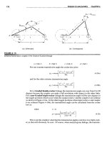
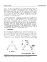
Fig. 2.1.1 Coordinate systems for two links connected by a revolute joint.

Note that the transfer matrix between the system of link i (i + 1) and the system of link
(i − 1)i is the inverse of [Ti ( i +1) ] . That is

[T ] = [T ]
( i +1) i

i ( i +1)

1


−1
ai ( i +1) Cθ i
=
 ai ( i +1) Sθ i

 Ri

0

Cθ i
Sθ i
0

0
− Cα i (i +1) Sθ i
Cα i ( i +1) Cθ i
− Sα i ( i +1)


Sα i ( i +1) Sθ i 
− Sα i ( i +1) Cθ i 

Cα i ( i +1) 
0

(2.1.5)

2.2 3D OVERCONSTRAINED LINKAGES

The minimum number of links to construct a mobile loop with revolute joints is four as
a loop with three links and three revolute joints is either a rigid structure or an
infinitesimal mechanism when all three revolute axes are coplanar and intersect at a
single point (Phillips, 1990). So 3D overconstrained linkages can have four, five or six

8


Chapter 2 Review of Previous Work
———————————————————————————————————

links. When these linkages consist of only revolute joints, they are called 4R, 5R or 6R
linkages.

The first overconstrained mechanism which appeared in the literature was proposed by
Sarrus (1853). Since then, other overconstrained mechanisms have been proposed by
various researchers. Of special interest are those proposed by Bennett (1903), Delassus
(1922), Bricard (1927), Myard (1931), Goldberg (1943), Waldron (1967, 1968 and
1969), Wohlhart (1987, 1991 and 1993) and Dietmaier (1995). Phillips (1984, 1990)
summarised all of the known overconstrained mechanisms in his two-volume book.
However, the most detailed studies of the subject of overconstraint in mechanisms are
due to Baker (1980, 1984, etc.).

2.2.1

4R Linkage - Bennett Linkage

Common 4R mobile loops can normally be classified into two types: the axes of rotation
are all parallel to one another, or they are concurrent, i.e. they intersect at a point,
leading to 2D 4R or spherical 4R linkages, respectively. Any disposition of the axes
different from these two special arrangements is known usually to be a chain of four
pieces which is, in general, completely rigid and so furnishes no mechanism at all. But
there is an exception, which is the Bennett linkage (Bennett, 1903).

The Bennett linkage is a skewed linkage of four pieces having the axes of revolute
joints neither parallel nor concurrent. Figure 2.2.1 shows the original model made by
Bennett. This linkage was also found independently by Borel (Bennett, 1914). Its

9

Chapter 2 Review of Previous Work
———————————————————————————————————
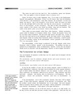
behaviour is better illustrated by the schematic diagram shown in Fig. 2.2.2. The four
links are connected by revolute joints, each of which has axis perpendicular to the two
adjacent links connected by it. The lengths of the links are given alongside the links,
and the twists are indicated at each joint. Bennett (1914) identified the conditions for the
linkage to have a single degree of mobility as follows.

Fig. 2.2.1 Original model of the Bennett linkage.

12

a23

3

2

2

a12

3

1

23

1

a34
a41

4

41

4
34

Fig. 2.2.2 A schematic diagram of the Bennett linkage.
Thick lines represent four links.
10