Design and analysis of experiments

Design and Analysis
of Experiments
Eighth Edition

DOUGLAS C. MONTGOMERY
Arizona State University

John Wiley & Sons, Inc.


VICE PRESIDENT AND PUBLISHER
ACQUISITIONS EDITOR
CONTENT MANAGER
PRODUCTION EDITOR
MARKETING MANAGER
DESIGN DIRECTOR
SENIOR DESIGNER
EDITORIAL ASSISTANT
PRODUCTION SERVICES
COVER PHOTO
COVER DESIGN

Donald Fowley
Linda Ratts
Lucille Buonocore
Anna Melhorn
Christopher Ruel
Harry Nolan
Maureen Eide
Christopher Teja

Namit Grover/Thomson Digital
Nik Wheeler/Corbis Images
Wendy Lai

This book was set in Times by Thomson Digital and printed and bound by Courier Westford.
The cover was printed by Courier Westford.
This book is printed on acid-free paper. ȍ
Founded in 1807, John Wiley & Sons, Inc. has been a valued source of knowledge and understanding for more
than 200 years, helping people around the world meet their needs and fulfill their aspirations. Our company is built
on a foundation of principles that include responsibility to the communities we serve and where we live and work.
In 2008, we launched a Corporate Citizenship Initiative, a global effort to address the environmental, social,
economic, and ethical challenges we face in our business. Among the issues we are addressing are carbon impact,
paper specifications and procurement, ethical conduct within our business and among our vendors, and community
and charitable support. For more information, please visit our website: www.wiley.com/go/citizenship.
Copyright © 2013, 2009, 2005, 2001, 1997 John Wiley & Sons, Inc. All rights reserved. No part of this publication
may be reproduced, stored in a retrieval system or transmitted in any form or by any means, electronic, mechanical,
photocopying, recording, scanning or otherwise, except as permitted under Sections 107 or 108 of the 1976
United States Copyright Act, without either the prior written permission of the Publisher, or authorization through
payment of the appropriate per-copy fee to the Copyright Clearance Center, Inc., 222 Rosewood Drive, Danvers,
MA 01923, website www.copyright.com. Requests to the Publisher for permission should be addressed to the
Permissions Department, John Wiley & Sons, Inc., 111 River Street, Hoboken, NJ 07030-5774, (201) 748-6011,
fax (201) 748-6008, website www.wiley.com/go/permissions.
Evaluation copies are provided to qualified academics and professionals for review purposes only, for use in their
courses during the next academic year. These copies are licensed and may not be sold or transferred to a third
party. Upon completion of the review period, please return the evaluation copy to Wiley. Return instructions and a
free of charge return shipping label are available at www.wiley.com/go/returnlabel. Outside of the United States,
please contact your local representative.
To order books or for customer service, please call 1-800-CALL WILEY (225-5945).
Library of Congress Cataloging-in-Publication Data:
Montgomery, Douglas C.

Design and analysis of experiments / Douglas C. Montgomery. — Eighth edition.
pages cm
Includes bibliographical references and index.
ISBN 978-1-118-14692-7
1. Experimental design. I. Title.
QA279.M66 2013
519.5'7—dc23
2012000877
ISBN 978-1118-14692-7
10 9 8 7 6 5 4 3 2 1


Preface

Audience
This is an introductory textbook dealing with the design and analysis of experiments. It is based
on college-level courses in design of experiments that I have taught over nearly 40 years at
Arizona State University, the University of Washington, and the Georgia Institute of Technology.
It also reflects the methods that I have found useful in my own professional practice as an engineering and statistical consultant in many areas of science and engineering, including the research
and development activities required for successful technology commercialization and product
realization.
The book is intended for students who have completed a first course in statistical methods. This background course should include at least some techniques of descriptive statistics,
the standard sampling distributions, and an introduction to basic concepts of confidence
intervals and hypothesis testing for means and variances. Chapters 10, 11, and 12 require
some familiarity with matrix algebra.
Because the prerequisites are relatively modest, this book can be used in a second course
on statistics focusing on statistical design of experiments for undergraduate students in engineering, the physical and chemical sciences, statistics, mathematics, and other fields of science.
For many years I have taught a course from the book at the first-year graduate level in engineering. Students in this course come from all of the fields of engineering, materials science,
physics, chemistry, mathematics, operations research life sciences, and statistics. I have also
used this book as the basis of an industrial short course on design of experiments for practicing technical professionals with a wide variety of backgrounds. There are numerous examples

illustrating all of the design and analysis techniques. These examples are based on real-world
applications of experimental design and are drawn from many different fields of engineering and
the sciences. This adds a strong applications flavor to an academic course for engineers
and scientists and makes the book useful as a reference tool for experimenters in a variety
of disciplines.

v


vi

Preface

About the Book
The eighth edition is a major revision of the book. I have tried to maintain the balance
between design and analysis topics of previous editions; however, there are many new topics
and examples, and I have reorganized much of the material. There is much more emphasis on
the computer in this edition.

Design-Expert, JMP, and Minitab Software
During the last few years a number of excellent software products to assist experimenters in
both the design and analysis phases of this subject have appeared. I have included output from
three of these products, Design-Expert, JMP, and Minitab at many points in the text. Minitab
and JMP are widely available general-purpose statistical software packages that have good
data analysis capabilities and that handles the analysis of experiments with both fixed and random factors (including the mixed model). Design-Expert is a package focused exclusively on
experimental design. All three of these packages have many capabilities for construction and
evaluation of designs and extensive analysis features. Student versions of Design-Expert and
JMP are available as a packaging option with this book, and their use is highly recommended. I urge all instructors who use this book to incorporate computer software into your
course. (In my course, I bring a laptop computer and use a computer projector in every
lecture, and every design or analysis topic discussed in class is illustrated with the computer.)

To request this book with the student version of JMP or Design-Expert included, contact
your local Wiley representative. You can find your local Wiley representative by going to
www.wiley.com/college and clicking on the tab for “Who’s My Rep?”

Empirical Model
I have continued to focus on the connection between the experiment and the model that
the experimenter can develop from the results of the experiment. Engineers (and physical,
chemical and life scientists to a large extent) learn about physical mechanisms and their
underlying mechanistic models early in their academic training, and throughout much of
their professional careers they are involved with manipulation of these models.
Statistically designed experiments offer the engineer a valid basis for developing an
empirical model of the system being investigated. This empirical model can then be
manipulated (perhaps through a response surface or contour plot, or perhaps mathematically) just as any other engineering model. I have discovered through many years of teaching
that this viewpoint is very effective in creating enthusiasm in the engineering community
for statistically designed experiments. Therefore, the notion of an underlying empirical
model for the experiment and response surfaces appears early in the book and receives
much more emphasis.

Factorial Designs
I have expanded the material on factorial and fractional factorial designs (Chapters 5 – 9) in
an effort to make the material flow more effectively from both the reader’s and the instructor’s viewpoint and to place more emphasis on the empirical model. There is new material
on a number of important topics, including follow-up experimentation following a fractional
factorial, nonregular and nonorthogonal designs, and small, efficient resolution IV and V
designs. Nonregular fractions as alternatives to traditional minimum aberration fractions in
16 runs and analysis methods for these design are discussed and illustrated.


Preface

vii

Additional Important Changes
I have added a lot of material on optimal designs and their application. The chapter on response
surfaces (Chapter 11) has several new topics and problems. I have expanded Chapter 12 on
robust parameter design and process robustness experiments. Chapters 13 and 14 discuss
experiments involving random effects and some applications of these concepts to nested and
split-plot designs. The residual maximum likelihood method is now widely available in software and I have emphasized this technique throughout the book. Because there is expanding
industrial interest in nested and split-plot designs, Chapters 13 and 14 have several new topics.
Chapter 15 is an overview of important design and analysis topics: nonnormality of the
response, the Box – Cox method for selecting the form of a transformation, and other alternatives; unbalanced factorial experiments; the analysis of covariance, including covariates in a
factorial design, and repeated measures. I have also added new examples and problems from
various fields, including biochemistry and biotechnology.

Experimental Design
Throughout the book I have stressed the importance of experimental design as a tool for engineers and scientists to use for product design and development as well as process development and improvement. The use of experimental design in developing products that are robust
to environmental factors and other sources of variability is illustrated. I believe that the use of
experimental design early in the product cycle can substantially reduce development lead time
and cost, leading to processes and products that perform better in the field and have higher
reliability than those developed using other approaches.
The book contains more material than can be covered comfortably in one course, and I
hope that instructors will be able to either vary the content of each course offering or discuss
some topics in greater depth, depending on class interest. There are problem sets at the end
of each chapter. These problems vary in scope from computational exercises, designed to
reinforce the fundamentals, to extensions or elaboration of basic principles.

Course Suggestions
My own course focuses extensively on factorial and fractional factorial designs. Consequently,
I usually cover Chapter 1, Chapter 2 (very quickly), most of Chapter 3, Chapter 4 (excluding
the material on incomplete blocks and only mentioning Latin squares briefly), and I discuss
Chapters 5 through 8 on factorials and two-level factorial and fractional factorial designs in

detail. To conclude the course, I introduce response surface methodology (Chapter 11) and give
an overview of random effects models (Chapter 13) and nested and split-plot designs (Chapter
14). I always require the students to complete a term project that involves designing, conducting, and presenting the results of a statistically designed experiment. I require them to do this
in teams because this is the way that much industrial experimentation is conducted. They must
present the results of this project, both orally and in written form.

The Supplemental Text Material
For the eighth edition I have prepared supplemental text material for each chapter of the book.
Often, this supplemental material elaborates on topics that could not be discussed in greater detail
in the book. I have also presented some subjects that do not appear directly in the book, but an
introduction to them could prove useful to some students and professional practitioners. Some of
this material is at a higher mathematical level than the text. I realize that instructors use this book


viii

Preface

with a wide array of audiences, and some more advanced design courses could possibly benefit
from including several of the supplemental text material topics. This material is in electronic form
on the World Wide Website for this book, located at www.wiley.com/college/montgomery.

Website
Current supporting material for instructors and students is available at the website
www.wiley.com/college/montgomery. This site will be used to communicate information
about innovations and recommendations for effectively using this text. The supplemental text
material described above is available at the site, along with electronic versions of data sets
used for examples and homework problems, a course syllabus, and some representative student term projects from the course at Arizona State University.

Student Companion Site

The student’s section of the textbook website contains the following:
1. The supplemental text material described above
2. Data sets from the book examples and homework problems, in electronic form
3. Sample Student Projects

Instructor Companion Site
The instructor’s section of the textbook website contains the following:
4.
5.
6.
7.
8.
9.
10.

Solutions to the text problems
The supplemental text material described above
PowerPoint lecture slides
Figures from the text in electronic format, for easy inclusion in lecture slides
Data sets from the book examples and homework problems, in electronic form
Sample Syllabus
Sample Student Projects

The instructor’s section is for instructor use only, and is password-protected. Visit the
Instructor Companion Site portion of the website, located at www.wiley.com/college/
montgomery, to register for a password.

Student Solutions Manual
The purpose of the Student Solutions Manual is to provide the student with an in-depth understanding of how to apply the concepts presented in the textbook. Along with detailed instructions on how to solve the selected chapter exercises, insights from practical applications are
also shared.

Solutions have been provided for problems selected by the author of the text.
Occasionally a group of “continued exercises” is presented and provides the student with a
full solution for a specific data set. Problems that are included in the Student Solutions
Manual are indicated by an icon appearing in the text margin next to the problem statement.
This is an excellent study aid that many text users will find extremely helpful. The
Student Solutions Manual may be ordered in a set with the text, or purchased separately.
Contact your local Wiley representative to request the set for your bookstore, or purchase the
Student Solutions Manual from the Wiley website.


Preface

ix

Acknowledgments
I express my appreciation to the many students, instructors, and colleagues who have used the six
earlier editions of this book and who have made helpful suggestions for its revision. The contributions of Dr. Raymond H. Myers, Dr. G. Geoffrey Vining, Dr. Brad Jones,
Dr. Christine Anderson-Cook, Dr. Connie M. Borror, Dr. Scott Kowalski, Dr. Dennis Lin,
Dr. John Ramberg, Dr. Joseph Pignatiello, Dr. Lloyd S. Nelson, Dr. Andre Khuri, Dr. Peter
Nelson, Dr. John A. Cornell, Dr. Saeed Maghsoodlo, Dr. Don Holcomb, Dr. George C. Runger,
Dr. Bert Keats, Dr. Dwayne Rollier, Dr. Norma Hubele, Dr. Murat Kulahci, Dr. Cynthia Lowry,
Dr. Russell G. Heikes, Dr. Harrison M. Wadsworth, Dr. William W. Hines, Dr. Arvind Shah,
Dr. Jane Ammons, Dr. Diane Schaub, Mr. Mark Anderson, Mr. Pat Whitcomb, Dr. Pat Spagon,
and Dr. William DuMouche were particularly valuable. My current and former Department
Chairs, Dr. Ron Askin and Dr. Gary Hogg, have provided an intellectually stimulating environment in which to work.
The contributions of the professional practitioners with whom I have worked have been
invaluable. It is impossible to mention everyone, but some of the major contributors include
Dr. Dan McCarville of Mindspeed Corporation, Dr. Lisa Custer of the George Group;
Dr. Richard Post of Intel; Mr. Tom Bingham, Mr. Dick Vaughn, Dr. Julian Anderson,
Mr. Richard Alkire, and Mr. Chase Neilson of the Boeing Company; Mr. Mike Goza, Mr. Don

Walton, Ms. Karen Madison, Mr. Jeff Stevens, and Mr. Bob Kohm of Alcoa; Dr. Jay Gardiner,
Mr. John Butora, Mr. Dana Lesher, Mr. Lolly Marwah, Mr. Leon Mason of IBM; Dr. Paul
Tobias of IBM and Sematech; Ms. Elizabeth A. Peck of The Coca-Cola Company; Dr. Sadri
Khalessi and Mr. Franz Wagner of Signetics; Mr. Robert V. Baxley of Monsanto Chemicals;
Mr. Harry Peterson-Nedry and Dr. Russell Boyles of Precision Castparts Corporation;
Mr. Bill New and Mr. Randy Schmid of Allied-Signal Aerospace; Mr. John M. Fluke, Jr. of
the John Fluke Manufacturing Company; Mr. Larry Newton and Mr. Kip Howlett of GeorgiaPacific; and Dr. Ernesto Ramos of BBN Software Products Corporation.
I am indebted to Professor E. S. Pearson and the Biometrika Trustees, John Wiley &
Sons, Prentice Hall, The American Statistical Association, The Institute of Mathematical
Statistics, and the editors of Biometrics for permission to use copyrighted material. Dr. Lisa
Custer and Dr. Dan McCorville did an excellent job of preparing the solutions that appear in
the Instructor’s Solutions Manual, and Dr. Cheryl Jennings and Dr. Sarah Streett provided
effective and very helpful proofreading assistance. I am grateful to NASA, the Office of
Naval Research, the National Science Foundation, the member companies of the
NSF/Industry/University Cooperative Research Center in Quality and Reliability Engineering
at Arizona State University, and the IBM Corporation for supporting much of my research
in engineering statistics and experimental design.
DOUGLAS C. MONTGOMERY
TEMPE, ARIZONA



Contents

Preface

v

1

Introduction

1

1.1
1.2
1.3
1.4
1.5
1.6
1.7

1
8
11
14
21
22
23

Strategy of Experimentation
Some Typical Applications of Experimental Design
Basic Principles
Guidelines for Designing Experiments
A Brief History of Statistical Design
Summary: Using Statistical Techniques in Experimentation
Problems

2

Simple Comparative Experiments
2.1
2.2
2.3
2.4

2.5
2.6
2.7

25

Introduction
Basic Statistical Concepts
Sampling and Sampling Distributions
Inferences About the Differences in Means, Randomized Designs

25
27
30
36

2.4.1
2.4.2
2.4.3
2.4.4
2.4.5
2.4.6
2.4.7

36
43
44
48
50
50
51

Hypothesis Testing
Confidence Intervals
Choice of Sample Size
The Case Where ␴21 Z ␴22
The Case Where ␴21 and ␴22 Are Known
Comparing a Single Mean to a Specified Value
Summary

Inferences About the Differences in Means, Paired Comparison Designs

53

2.5.1
2.5.2

The Paired Comparison Problem
Advantages of the Paired Comparison Design

53
56

Inferences About the Variances of Normal Distributions

Problems

57
59

xi


xii

Contents

3

Experiments with a Single Factor:
The Analysis of Variance
3.1
3.2
3.3

3.4

3.5

An Example
The Analysis of Variance
Analysis of the Fixed Effects Model

66
68

70

3.3.1
3.3.2
3.3.3
3.3.4

71
73
78
79

3.8

3.9

Decomposition of the Total Sum of Squares
Statistical Analysis
Estimation of the Model Parameters
Unbalanced Data

Model Adequacy Checking

80

3.4.1
3.4.2
3.4.3
3.4.4

80
82
83
88

The Normality Assumption
Plot of Residuals in Time Sequence
Plot of Residuals Versus Fitted Values
Plots of Residuals Versus Other Variables

Practical Interpretation of Results
3.5.1
3.5.2
3.5.3
3.5.4
3.5.5
3.5.6
3.5.7
3.5.8

3.6
3.7

65

A Regression Model
Comparisons Among Treatment Means
Graphical Comparisons of Means
Contrasts
Orthogonal Contrasts

Scheffé’s Method for Comparing All Contrasts
Comparing Pairs of Treatment Means
Comparing Treatment Means with a Control

89
89
90
91
92
94
96
97
101

Sample Computer Output
Determining Sample Size

102
105

3.7.1
3.7.2
3.7.3

105
108
109

Operating Characteristic Curves
Specifying a Standard Deviation Increase

Confidence Interval Estimation Method

Other Examples of Single-Factor Experiments

110

3.8.1
3.8.2
3.8.3

110
110
114

Chocolate and Cardiovascular Health
A Real Economy Application of a Designed Experiment
Discovering Dispersion Effects

The Random Effects Model

116

3.9.1
3.9.2
3.9.3

116
117
118

A Single Random Factor
Analysis of Variance for the Random Model
Estimating the Model Parameters

3.10 The Regression Approach to the Analysis of Variance

125

3.10.1 Least Squares Estimation of the Model Parameters
3.10.2 The General Regression Significance Test

125
126

3.11 Nonparametric Methods in the Analysis of Variance
3.11.1 The Kruskal–Wallis Test
3.11.2 General Comments on the Rank Transformation

3.12 Problems

128
128
130

130

4

Randomized Blocks, Latin Squares,
and Related Designs

4 . 1 The Randomized Complete Block Design
4.1.1
4.1.2

Statistical Analysis of the RCBD
Model Adequacy Checking

139
139
141
149


Contents

4.1.3
4.1.4

4.2
4.3
4.4

4.5

Some Other Aspects of the Randomized Complete Block Design
Estimating Model Parameters and the General Regression
Significance Test

4.4.1
4.4.2

4.4.3

168
172
174
177

Statistical Analysis of the BIBD
Least Squares Estimation of the Parameters
Recovery of Interblock Information in the BIBD

Problems

183

Basic Definitions and Principles
The Advantage of Factorials
The Two-Factor Factorial Design

183
186
187

5.3.1
5.3.2
5.3.3
5.3.4
5.3.5
5.3.6
5.3.7

187
189
198
198
201
202
203

An Example
Statistical Analysis of the Fixed Effects Model
Model Adequacy Checking
Estimating the Model Parameters
Choice of Sample Size
The Assumption of No Interaction in a Two-Factor Model
One Observation per Cell

The General Factorial Design
Fitting Response Curves and Surfaces
Blocking in a Factorial Design
Problems

6

The 2k Factorial Design
6.1
6.2
6.3
6.4
6.5

6.6
6.7
6.8
6.9
6.10

155

158
165
168

Introduction to Factorial Designs

5.4
5.5
5.6
5.7

150

The Latin Square Design
The Graeco-Latin Square Design
Balanced Incomplete Block Designs

5
5.1
5.2
5.3

xiii

Introduction
The 22 Design
The 23 Design
The General 2k Design
A Single Replicate of the 2k Design
Additional Examples of Unreplicated 2k Design
2k Designs are Optimal Designs
The Addition of Center Points to the 2k Design
Why We Work with Coded Design Variables
Problems

206
211
219
225

233
233
234
241
253
255
268
280
285
290
292

7

Blocking and Confounding in the 2k
Factorial Design
7.1
7.2
7.3

Introduction
Blocking a Replicated 2k Factorial Design
Confounding in the 2k Factorial Design

304
304
305
306


xiv

Contents

7.4
7.5
7.6
7.7
7.8
7.9

Confounding the 2k Factorial Design in Two Blocks

Another Illustration of Why Blocking Is Important
Confounding the 2k Factorial Design in Four Blocks
Confounding the 2k Factorial Design in 2p Blocks
Partial Confounding
Problems

8

Two-Level Fractional Factorial Designs
8.1
8.2

8.3
8.4

8.5
8.6

320

Introduction
The One-Half Fraction of the 2k Design

320
321

8.2.1
8.2.2
8.2.3

321
323
324

Definitions and Basic Principles
Design Resolution
Construction and Analysis of the One-Half Fraction

The One-Quarter Fraction of the 2k Design
The General 2kϪp Fractional Factorial Design

333
340

8.4.1
8.4.2
8.4.3

340
343
344

Choosing a Design
Analysis of 2kϪp Fractional Factorials
Blocking Fractional Factorials

Alias Structures in Fractional Factorials
and other Designs
Resolution III Designs
8.6.1

8.6.2

Constructing Resolution III Designs
Fold Over of Resolution III Fractions to
Separate Aliased Effects
Plackett-Burman Designs

8.6.3

8.7

306
312
313
315
316
319

349
351
351
353
357

Resolution IV and V Designs

366

8.7.1
8.7.2

8.7.3

366
367
373

Resolution IV Designs
Sequential Experimentation with Resolution IV Designs
Resolution V Designs

8.8 Supersaturated Designs
8.9 Summary
8.10 Problems

374
375
376

9

Additional Design and Analysis Topics for Factorial
and Fractional Factorial Designs
9.1

k

The 3 Factorial Design
9.1.1
9.1.2
9.1.3

9.1.4

9.2

Confounding in the 3k Factorial Design
9.2.1
9.2.2
9.2.3

9.3

Notation and Motivation for the 3k Design
The 32 Design
The 33 Design
The General 3k Design
The 3k Factorial Design in Three Blocks
The 3k Factorial Design in Nine Blocks
The 3k Factorial Design in 3p Blocks

Fractional Replication of the 3k Factorial Design
9.3.1
9.3.2

The One-Third Fraction of the 3k Factorial Design
Other 3kϪp Fractional Factorial Designs

394
395
395
396

397
402

402
403
406
407

408
408
410


Contents

9.4
9.5

9.6

9.7

Factorials with Mixed Levels

412

9.4.1
9.4.2

412

414

Factors at Two and Three Levels
Factors at Two and Four Levels

Nonregular Fractional Factorial Designs

415

9.5.1 Nonregular Fractional Factorial Designs for 6, 7, and 8 Factors in 16 Runs
9.5.2 Nonregular Fractional Factorial Designs for 9 Through 14 Factors in 16 Runs
9.5.3 Analysis of Nonregular Fractional Factorial Designs

418
425
427

Constructing Factorial and Fractional Factorial Designs Using
an Optimal Design Tool

431

9.6.1
9.6.2
9.6.3

433
433
443

Design Optimality Criteria
Examples of Optimal Designs
Extensions of the Optimal Design Approach

Problems

10

Fitting Regression Models
10.1
10.2
10.3
10.4

444

449

Introduction
Linear Regression Models
Estimation of the Parameters in Linear Regression Models
Hypothesis Testing in Multiple Regression

449
450
451
462

10.4.1 Test for Significance of Regression
10.4.2 Tests on Individual Regression Coefficients and Groups of Coefficients

462
464

10.5 Confidence Intervals in Multiple Regression
10.5.1 Confidence Intervals on the Individual Regression Coefficients
10.5.2 Confidence Interval on the Mean Response

10.6 Prediction of New Response Observations
10.7 Regression Model Diagnostics
10.7.1 Scaled Residuals and PRESS
10.7.2 Influence Diagnostics

10.8 Testing for Lack of Fit
10.9 Problems

11

Response Surface Methods and Designs
11.1 Introduction to Response Surface Methodology
11.2 The Method of Steepest Ascent
11.3 Analysis of a Second-Order Response Surface
11.3.1
11.3.2
11.3.3
11.3.4

Location of the Stationary Point
Characterizing the Response Surface
Ridge Systems

Multiple Responses

11.4 Experimental Designs for Fitting Response Surfaces
11.4.1
11.4.2
11.4.3
11.4.4

11.5
11.6
11.7
11.8

xv

Designs for Fitting the First-Order Model
Designs for Fitting the Second-Order Model
Blocking in Response Surface Designs
Optimal Designs for Response Surfaces

Experiments with Computer Models
Mixture Experiments
Evolutionary Operation
Problems

467
467
468

468

470
470
472

473
475

478
478
480
486
486
488
495
496

500
501
501
507
511

523
530
540
544


xvi

Contents

12

Robust Parameter Design and Process
Robustness Studies
12.1
12.2
12.3
12.4

Introduction
Crossed Array Designs
Analysis of the Crossed Array Design
Combined Array Designs and the Response
Model Approach
12.5 Choice of Designs
12.6 Problems

13

Experiments with Random Factors
13.1
13.2
13.3
13.4
13.5
13.6
13.7

554
556
558
561
567
570

573

Random Effects Models
The Two-Factor Factorial with Random Factors
The Two-Factor Mixed Model
Sample Size Determination with Random Effects
Rules for Expected Mean Squares
Approximate F Tests
Some Additional Topics on Estimation of Variance Components

573
574
581
587
588
592
596

13.7.1 Approximate Confidence Intervals on Variance Components
13.7.2 The Modified Large-Sample Method

597
600

13.8 Problems

14

Nested and Split-Plot Designs
14.1 The Two-Stage Nested Design
14.1.1
14.1.2
14.1.3
14.1.4

14.2
14.3
14.4
14.5

554

Statistical Analysis
Diagnostic Checking
Variance Components
Staggered Nested Designs

601

604
604
605
609

611
612

The General m-Stage Nested Design
Designs with Both Nested and Factorial Factors
The Split-Plot Design
Other Variations of the Split-Plot Design

614
616
621
627

14.5.1 Split-Plot Designs with More Than Two Factors
14.5.2 The Split-Split-Plot Design
14.5.3 The Strip-Split-Plot Design

627
632
636

14.6 Problems

15

Other Design and Analysis Topics
15.1 Nonnormal Responses and Transformations
15.1.1 Selecting a Transformation: The Box–Cox Method
15.1.2 The Generalized Linear Model

637

642
643
643
645


Contents

15.2 Unbalanced Data in a Factorial Design
15.2.1 Proportional Data: An Easy Case
15.2.2 Approximate Methods
15.2.3 The Exact Method

15.3 The Analysis of Covariance
15.3.1
15.3.2
15.3.3
15.3.4

Description of the Procedure
Computer Solution
Development by the General Regression Significance Test
Factorial Experiments with Covariates

15.4 Repeated Measures
15.5 Problems

Appendix

Table I.
Table II.
Table III.
Table IV.
Table V.
Table VI.
Table VII.
Table VIII.
Table IX.
Table X.

xvii
652
652
654
655

655
656
664
665
667

677
679

683
Cumulative Standard Normal Distribution
Percentage Points of the t Distribution
Percentage Points of the ␹2 Distribution

Percentage Points of the F Distribution
Operating Characteristic Curves for the Fixed Effects Model
Analysis of Variance
Operating Characteristic Curves for the Random Effects Model
Analysis of Variance
Percentage Points of the Studentized Range Statistic
Critical Values for Dunnett’s Test for Comparing Treatments
with a Control
Coefficients of Orthogonal Polynomials
Alias Relationships for 2kϪp Fractional Factorial Designs with k Յ 15
and n Յ 64

684
686
687
688
693
697
701
703
705
706

Bibliography

719

Index

725

C H A P T E R

1

Introduction
CHAPTER OUTLINE
1.1 STRATEGY OF EXPERIMENTATION
1.2 SOME TYPICAL APPLICATIONS
OF EXPERIMENTAL DESIGN
1.3 BASIC PRINCIPLES
1.4 GUIDELINES FOR DESIGNING EXPERIMENTS
1.5 A BRIEF HISTORY OF STATISTICAL DESIGN
1.6 SUMMARY: USING STATISTICAL TECHNIQUES
IN EXPERIMENTATION

SUPPLEMENTAL MATERIAL FOR CHAPTER 1
S1.1 More about Planning Experiments
S1.2 Blank Guide Sheets to Assist in Pre-Experimental
Planning
S1.3 Montgomery’s Theorems on Designed Experiments

The supplemental material is on the textbook website www.wiley.com/college/montgomery.

1.1

Strategy of Experimentation
Observing a system or process while it is in operation is an important part of the learning
process, and is an integral part of understanding and learning about how systems and

processes work. The great New York Yankees catcher Yogi Berra said that “. . . you can
observe a lot just by watching.” However, to understand what happens to a process when
you change certain input factors, you have to do more than just watch—you actually have
to change the factors. This means that to really understand cause-and-effect relationships in
a system you must deliberately change the input variables to the system and observe the
changes in the system output that these changes to the inputs produce. In other words, you
need to conduct experiments on the system. Observations on a system or process can lead
to theories or hypotheses about what makes the system work, but experiments of the type
described above are required to demonstrate that these theories are correct.
Investigators perform experiments in virtually all fields of inquiry, usually to discover
something about a particular process or system. Each experimental run is a test. More formally,
we can define an experiment as a test or series of runs in which purposeful changes are made
to the input variables of a process or system so that we may observe and identify the reasons
for changes that may be observed in the output response. We may want to determine which
input variables are responsible for the observed changes in the response, develop a model
relating the response to the important input variables and to use this model for process or system
improvement or other decision-making.
This book is about planning and conducting experiments and about analyzing the
resulting data so that valid and objective conclusions are obtained. Our focus is on experiments in engineering and science. Experimentation plays an important role in technology

1


2

Chapter 1 ■ Introduction

commercialization and product realization activities, which consist of new product design
and formulation, manufacturing process development, and process improvement. The objective in many cases may be to develop a robust process, that is, a process affected minimally
by external sources of variability. There are also many applications of designed experiments

in a nonmanufacturing or non-product-development setting, such as marketing, service operations, and general business operations.
As an example of an experiment, suppose that a metallurgical engineer is interested in
studying the effect of two different hardening processes, oil quenching and saltwater
quenching, on an aluminum alloy. Here the objective of the experimenter (the engineer) is
to determine which quenching solution produces the maximum hardness for this particular
alloy. The engineer decides to subject a number of alloy specimens or test coupons to each
quenching medium and measure the hardness of the specimens after quenching. The average hardness of the specimens treated in each quenching solution will be used to determine
which solution is best.
As we consider this simple experiment, a number of important questions come to mind:
1. Are these two solutions the only quenching media of potential interest?
2. Are there any other factors that might affect hardness that should be investigated or
controlled in this experiment (such as, the temperature of the quenching media)?
3. How many coupons of alloy should be tested in each quenching solution?
4. How should the test coupons be assigned to the quenching solutions, and in what
order should the data be collected?
5. What method of data analysis should be used?
6. What difference in average observed hardness between the two quenching media
will be considered important?
All of these questions, and perhaps many others, will have to be answered satisfactorily
before the experiment is performed.
Experimentation is a vital part of the scientific (or engineering) method. Now there are
certainly situations where the scientific phenomena are so well understood that useful results
including mathematical models can be developed directly by applying these well-understood
principles. The models of such phenomena that follow directly from the physical mechanism
are usually called mechanistic models. A simple example is the familiar equation for current
flow in an electrical circuit, Ohm’s law, E ϭ IR. However, most problems in science and engineering require observation of the system at work and experimentation to elucidate information about why and how it works. Well-designed experiments can often lead to a model of
system performance; such experimentally determined models are called empirical models.
Throughout this book, we will present techniques for turning the results of a designed experiment into an empirical model of the system under study. These empirical models can be
manipulated by a scientist or an engineer just as a mechanistic model can.
A well-designed experiment is important because the results and conclusions that can

be drawn from the experiment depend to a large extent on the manner in which the data were
collected. To illustrate this point, suppose that the metallurgical engineer in the above experiment used specimens from one heat in the oil quench and specimens from a second heat in
the saltwater quench. Now, when the mean hardness is compared, the engineer is unable to
say how much of the observed difference is the result of the quenching media and how much
is the result of inherent differences between the heats.1 Thus, the method of data collection
has adversely affected the conclusions that can be drawn from the experiment.
1

A specialist in experimental design would say that the effect of quenching media and heat were confounded; that is, the effects of
these two factors cannot be separated.


1.1 Strategy of Experimentation

FIGURE 1.1
process or system

Controllable factors
x1

Inputs

x2

z2

General model of a

Output
y

Process

z1

■

xp

3

zq

Uncontrollable factors

In general, experiments are used to study the performance of processes and systems.
The process or system can be represented by the model shown in Figure 1.1. We can usually
visualize the process as a combination of operations, machines, methods, people, and other
resources that transforms some input (often a material) into an output that has one or more
observable response variables. Some of the process variables and material properties x1,
x2, . . . , xp are controllable, whereas other variables z1, z2, . . . , zq are uncontrollable
(although they may be controllable for purposes of a test). The objectives of the experiment
may include the following:
1. Determining which variables are most influential on the response y
2. Determining where to set the influential x’s so that y is almost always near the
desired nominal value
3. Determining where to set the influential x’s so that variability in y is small
4. Determining where to set the influential x’s so that the effects of the uncontrollable
variables z1, z2, . . . , zq are minimized.
As you can see from the foregoing discussion, experiments often involve several factors.

Usually, an objective of the experimenter is to determine the influence that these factors have
on the output response of the system. The general approach to planning and conducting the
experiment is called the strategy of experimentation. An experimenter can use several strategies. We will illustrate some of these with a very simple example.
I really like to play golf. Unfortunately, I do not enjoy practicing, so I am always looking for a simpler solution to lowering my score. Some of the factors that I think may be important, or that may influence my golf score, are as follows:
1.
2.
3.
4.
5.
6.
7.
8.

The type of driver used (oversized or regular sized)
The type of ball used (balata or three piece)
Walking and carrying the golf clubs or riding in a golf cart
Drinking water or drinking “something else” while playing
Playing in the morning or playing in the afternoon
Playing when it is cool or playing when it is hot
The type of golf shoe spike worn (metal or soft)
Playing on a windy day or playing on a calm day.

Obviously, many other factors could be considered, but let’s assume that these are the ones of primary interest. Furthermore, based on long experience with the game, I decide that factors 5
through 8 can be ignored; that is, these factors are not important because their effects are so small


Chapter 1 ■ Introduction

R

O
Driver
■

FIGURE 1.2

T

B
Ball

Score

Score

Score

that they have no practical value. Engineers, scientists, and business analysts, often must make
these types of decisions about some of the factors they are considering in real experiments.
Now, let’s consider how factors 1 through 4 could be experimentally tested to determine
their effect on my golf score. Suppose that a maximum of eight rounds of golf can be played
over the course of the experiment. One approach would be to select an arbitrary combination
of these factors, test them, and see what happens. For example, suppose the oversized driver,
balata ball, golf cart, and water combination is selected, and the resulting score is 87. During
the round, however, I noticed several wayward shots with the big driver (long is not always
good in golf), and, as a result, I decide to play another round with the regular-sized driver,
holding the other factors at the same levels used previously. This approach could be continued almost indefinitely, switching the levels of one or two (or perhaps several) factors for the
next test, based on the outcome of the current test. This strategy of experimentation, which
we call the best-guess approach, is frequently used in practice by engineers and scientists. It
often works reasonably well, too, because the experimenters often have a great deal of technical or theoretical knowledge of the system they are studying, as well as considerable practical experience. The best-guess approach has at least two disadvantages. First, suppose the

initial best-guess does not produce the desired results. Now the experimenter has to take
another guess at the correct combination of factor levels. This could continue for a long time,
without any guarantee of success. Second, suppose the initial best-guess produces an acceptable result. Now the experimenter is tempted to stop testing, although there is no guarantee
that the best solution has been found.
Another strategy of experimentation that is used extensively in practice is the onefactor-at-a-time (OFAT) approach. The OFAT method consists of selecting a starting point,
or baseline set of levels, for each factor, and then successively varying each factor over its
range with the other factors held constant at the baseline level. After all tests are performed,
a series of graphs are usually constructed showing how the response variable is affected by
varying each factor with all other factors held constant. Figure 1.2 shows a set of these graphs
for the golf experiment, using the oversized driver, balata ball, walking, and drinking water
levels of the four factors as the baseline. The interpretation of this graph is straightforward;
for example, because the slope of the mode of travel curve is negative, we would conclude
that riding improves the score. Using these one-factor-at-a-time graphs, we would select the
optimal combination to be the regular-sized driver, riding, and drinking water. The type of
golf ball seems unimportant.
The major disadvantage of the OFAT strategy is that it fails to consider any possible
interaction between the factors. An interaction is the failure of one factor to produce the same
effect on the response at different levels of another factor. Figure 1.3 shows an interaction
between the type of driver and the beverage factors for the golf experiment. Notice that if I use
the regular-sized driver, the type of beverage consumed has virtually no effect on the score, but
if I use the oversized driver, much better results are obtained by drinking water instead of beer.
Interactions between factors are very common, and if they occur, the one-factor-at-a-time strategy will usually produce poor results. Many people do not recognize this, and, consequently,

Score

4

R
W
Mode of travel

SE
W
Beverage

Results of the one-factor-at-a-time strategy for the golf experiment


1.1 Strategy of Experimentation

T
Type of ball

Score

Oversized
driver

5

Regular-sized
driver

B
B

W

R

O

Beverage type

Type of driver

F I G U R E 1 . 3 Interaction between
type of driver and type of beverage for
the golf experiment

■

F I G U R E 1 . 4 A two-factor
factorial experiment involving type
of driver and type of ball

■

OFAT experiments are run frequently in practice. (Some individuals actually think that this
strategy is related to the scientific method or that it is a “sound” engineering principle.) Onefactor-at-a-time experiments are always less efficient than other methods based on a statistical
approach to design. We will discuss this in more detail in Chapter 5.
The correct approach to dealing with several factors is to conduct a factorial experiment. This is an experimental strategy in which factors are varied together, instead of one
at a time. The factorial experimental design concept is extremely important, and several
chapters in this book are devoted to presenting basic factorial experiments and a number of
useful variations and special cases.
To illustrate how a factorial experiment is conducted, consider the golf experiment and
suppose that only two factors, type of driver and type of ball, are of interest. Figure 1.4 shows
a two-factor factorial experiment for studying the joint effects of these two factors on my golf
score. Notice that this factorial experiment has both factors at two levels and that all possible
combinations of the two factors across their levels are used in the design. Geometrically, the

four runs form the corners of a square. This particular type of factorial experiment is called a
22 factorial design (two factors, each at two levels). Because I can reasonably expect to play
eight rounds of golf to investigate these factors, a reasonable plan would be to play two
rounds of golf at each combination of factor levels shown in Figure 1.4. An experimental
designer would say that we have replicated the design twice. This experimental design would
enable the experimenter to investigate the individual effects of each factor (or the main
effects) and to determine whether the factors interact.
Figure 1.5a shows the results of performing the factorial experiment in Figure 1.4. The
scores from each round of golf played at the four test combinations are shown at the corners
of the square. Notice that there are four rounds of golf that provide information about using
the regular-sized driver and four rounds that provide information about using the oversized
driver. By finding the average difference in the scores on the right- and left-hand sides of the
square (as in Figure 1.5b), we have a measure of the effect of switching from the oversized
driver to the regular-sized driver, or
92 ϩ 94 ϩ 93 ϩ 91 88 ϩ 91 ϩ 88 ϩ 90
Ϫ
4
4
ϭ 3.25

Driver effect ϭ

That is, on average, switching from the oversized to the regular-sized driver increases the
score by 3.25 strokes per round. Similarly, the average difference in the four scores at the top


Chapter 1 ■ Introduction

88, 91

92, 94

88, 90

93, 91

Type of ball

T

B

O

R
Type of driver

(a) Scores from the golf experiment
+
Type of ball
–

B

+

+

–

–

T

B

–

+

B

+

+

T

Type of ball

–
T
Type of ball

6

–

O
R

Type of driver

O
R
Type of driver

O
R
Type of driver

(b) Comparison of scores leading
to the driver effect

(c) Comparison of scores
leading to the ball effect

(d) Comparison of scores
leading to the ball–driver
interaction effect

FIGURE 1.5
factor effects

■

Scores from the golf experiment in Figure 1.4 and calculation of the

of the square and the four scores at the bottom measures the effect of the type of ball used
(see Figure 1.5c):
88 ϩ 91 ϩ 92 ϩ 94 88 ϩ 90 ϩ 93 ϩ 91

Ϫ
4
4
ϭ 0.75

Ball effect ϭ

Finally, a measure of the interaction effect between the type of ball and the type of driver can
be obtained by subtracting the average scores on the left-to-right diagonal in the square from
the average scores on the right-to-left diagonal (see Figure 1.5d), resulting in
92 ϩ 94 ϩ 88 ϩ 90 88 ϩ 91 ϩ 93 ϩ 91
Ϫ
4
4
ϭ 0.25

Ball–driver interaction effect ϭ

The results of this factorial experiment indicate that driver effect is larger than either the
ball effect or the interaction. Statistical testing could be used to determine whether any of
these effects differ from zero. In fact, it turns out that there is reasonably strong statistical evidence that the driver effect differs from zero and the other two effects do not. Therefore, this
experiment indicates that I should always play with the oversized driver.
One very important feature of the factorial experiment is evident from this simple
example; namely, factorials make the most efficient use of the experimental data. Notice that
this experiment included eight observations, and all eight observations are used to calculate
the driver, ball, and interaction effects. No other strategy of experimentation makes such an
efficient use of the data. This is an important and useful feature of factorials.
We can extend the factorial experiment concept to three factors. Suppose that I wish
to study the effects of type of driver, type of ball, and the type of beverage consumed on my
golf score. Assuming that all three factors have two levels, a factorial design can be set up

1.1 Strategy of Experimentation

7

FIGURE 1.6
A three-factor
factorial experiment involving type of
driver, type of ball, and type of beverage

Beverage

■

Ball
Driver

as shown in Figure 1.6. Notice that there are eight test combinations of these three factors
across the two levels of each and that these eight trials can be represented geometrically as
the corners of a cube. This is an example of a 23 factorial design. Because I only want to
play eight rounds of golf, this experiment would require that one round be played at each
combination of factors represented by the eight corners of the cube in Figure 1.6. However,
if we compare this to the two-factor factorial in Figure 1.4, the 23 factorial design would provide the same information about the factor effects. For example, there are four tests in both
designs that provide information about the regular-sized driver and four tests that provide
information about the oversized driver, assuming that each run in the two-factor design in
Figure 1.4 is replicated twice.
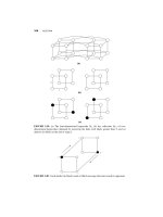
Figure 1.7 illustrates how all four factors—driver, ball, beverage, and mode of travel
(walking or riding)—could be investigated in a 24 factorial design. As in any factorial design,
all possible combinations of the levels of the factors are used. Because all four factors are at

two levels, this experimental design can still be represented geometrically as a cube (actually
a hypercube).
Generally, if there are k factors, each at two levels, the factorial design would require 2k
runs. For example, the experiment in Figure 1.7 requires 16 runs. Clearly, as the number of
factors of interest increases, the number of runs required increases rapidly; for instance, a
10-factor experiment with all factors at two levels would require 1024 runs. This quickly
becomes infeasible from a time and resource viewpoint. In the golf experiment, I can only
play eight rounds of golf, so even the experiment in Figure 1.7 is too large.
Fortunately, if there are four to five or more factors, it is usually unnecessary to run all
possible combinations of factor levels. A fractional factorial experiment is a variation of the
basic factorial design in which only a subset of the runs is used. Figure 1.8 shows a fractional
factorial design for the four-factor version of the golf experiment. This design requires only
8 runs instead of the original 16 and would be called a one-half fraction. If I can play only
eight rounds of golf, this is an excellent design in which to study all four factors. It will provide
good information about the main effects of the four factors as well as some information about
how these factors interact.

Mode of travel
Ride
Beverage

Walk

Ball
Driver

F I G U R E 1 . 7 A four-factor factorial experiment involving type
of driver, type of ball, type of beverage, and mode of travel

■

8

Chapter 1 ■ Introduction

Mode of travel
Ride
Beverage

Walk

Ball
Driver

F I G U R E 1 . 8 A four-factor fractional factorial experiment involving
type of driver, type of ball, type of beverage, and mode of travel

■

Fractional factorial designs are used extensively in industrial research and development,
and for process improvement. These designs will be discussed in Chapters 8 and 9.

1.2

Some Typical Applications of Experimental Design
Experimental design methods have found broad application in many disciplines. As noted
previously, we may view experimentation as part of the scientific process and as one of the
ways by which we learn about how systems or processes work. Generally, we learn through
a series of activities in which we make conjectures about a process, perform experiments to

generate data from the process, and then use the information from the experiment to establish
new conjectures, which lead to new experiments, and so on.
Experimental design is a critically important tool in the scientific and engineering
world for improving the product realization process. Critical components of these activities
are in new manufacturing process design and development, and process management. The
application of experimental design techniques early in process development can result in
1.
2.
3.
4.

Improved process yields
Reduced variability and closer conformance to nominal or target requirements
Reduced development time
Reduced overall costs.

Experimental design methods are also of fundamental importance in engineering
design activities, where new products are developed and existing ones improved. Some applications of experimental design in engineering design include
1. Evaluation and comparison of basic design configurations
2. Evaluation of material alternatives
3. Selection of design parameters so that the product will work well under a wide variety of field conditions, that is, so that the product is robust
4. Determination of key product design parameters that impact product performance
5. Formulation of new products.
The use of experimental design in product realization can result in products that are easier
to manufacture and that have enhanced field performance and reliability, lower product
cost, and shorter product design and development time. Designed experiments also have
extensive applications in marketing, market research, transactional and service operations,
and general business operations. We now present several examples that illustrate some of
these ideas.

1.2 Some Typical Applications of Experimental Design

EXAMPLE 1.1

Characterizing a Process

A flow solder machine is used in the manufacturing process
for printed circuit boards. The machine cleans the boards in
a flux, preheats the boards, and then moves them along a
conveyor through a wave of molten solder. This solder
process makes the electrical and mechanical connections
for the leaded components on the board.
The process currently operates around the 1 percent defective level. That is, about 1 percent of the solder joints on a
board are defective and require manual retouching. However,
because the average printed circuit board contains over 2000
solder joints, even a 1 percent defective level results in far too
many solder joints requiring rework. The process engineer
responsible for this area would like to use a designed experiment to determine which machine parameters are influential
in the occurrence of solder defects and which adjustments
should be made to those variables to reduce solder defects.
The flow solder machine has several variables that can
be controlled. They include
1.
2.
3.
4.
5.
6.
7.

Solder temperature
Preheat temperature
Conveyor speed
Flux type
Flux specific gravity
Solder wave depth
Conveyor angle.

In addition to these controllable factors, several other factors
cannot be easily controlled during routine manufacturing,
although they could be controlled for the purposes of a test.
They are
1. Thickness of the printed circuit board
2. Types of components used on the board

EXAMPLE 1.2

3. Layout of the components on the board
4. Operator
5. Production rate.
In this situation, engineers are interested in characterizing the flow solder machine; that is, they want to determine which factors (both controllable and uncontrollable)
affect the occurrence of defects on the printed circuit
boards. To accomplish this, they can design an experiment
that will enable them to estimate the magnitude and direction of the factor effects; that is, how much does the
response variable (defects per unit) change when each factor is changed, and does changing the factors together
produce different results than are obtained from individual
factor adjustments—that is, do the factors interact?
Sometimes we call an experiment such as this a screening
experiment. Typically, screening or characterization experiments involve using fractional factorial designs, such as in

the golf example in Figure 1.8.
The information from this screening or characterization
experiment will be used to identify the critical process factors and to determine the direction of adjustment for these
factors to reduce further the number of defects per unit. The
experiment may also provide information about which factors should be more carefully controlled during routine manufacturing to prevent high defect levels and erratic process
performance. Thus, one result of the experiment could be the
application of techniques such as control charts to one or
more process variables (such as solder temperature), in
addition to control charts on process output. Over time, if the
process is improved enough, it may be possible to base most
of the process control plan on controlling process input variables instead of control charting the output.

Optimizing a Process

In a characterization experiment, we are usually interested
in determining which process variables affect the response.
A logical next step is to optimize, that is, to determine the
region in the important factors that leads to the best possible response. For example, if the response is yield, we
would look for a region of maximum yield, whereas if the
response is variability in a critical product dimension, we
would seek a region of minimum variability.
Suppose that we are interested in improving the yield
of a chemical process. We know from the results of a characterization experiment that the two most important
process variables that influence the yield are operating
temperature and reaction time. The process currently runs

at 145°F and 2.1 hours of reaction time, producing yields
of around 80 percent. Figure 1.9 shows a view of the
time–temperature region from above. In this graph, the
lines of constant yield are connected to form response

contours, and we have shown the contour lines for yields
of 60, 70, 80, 90, and 95 percent. These contours are projections on the time–temperature region of cross sections
of the yield surface corresponding to the aforementioned
percent yields. This surface is sometimes called a
response surface. The true response surface in Figure 1.9
is unknown to the process personnel, so experimental
methods will be required to optimize the yield with
respect to time and temperature.

9