Excited states and photochemistry of organic molecules 1995 klessinger michl
Bạn đang xem bản rút gọn của tài liệu. Xem và tải ngay bản đầy đủ của tài liệu tại đây (27.15 MB, 281 trang )
Excited States and
Photochemistry
of
Organic Molecules
Martin Klessinger
WestBlische Wilhelms-Universitat Monster
Josef Michl
University of Colorado
+
VCH
Martin Klessinaer
Organisch-~hemischesInstitut
WestfMische Wilhelms-UnivenitBt
P48149 Monster
Germany
Josef Michl
Department of Chemistry and
Biochemistry
University of Colorado
Boulder, CO 80309-02 15
Library of Congress CaWoging-in-Publiestion Data
Klessinger. Martin.
Excited states and photochemistry of organic molecules I Martin
Klessinger, Josef Michl.
p.
cm.
Includes index.
ISBN 1-56081-588-4
1. Chemistry, Physical organic. 2. Photochemistry. 3. Excited
. 11. Title.
state chemistry. I. Michl, Josef, 1939QD476.K53 1994
547.1'354~20
92-46464
CIP
To our teachers
WOLFGANG
LUTTKE
RUDOLF
ZAHRADN~K
AND
8 1995 VCH Publishers, Inc.
This work is subject to copyright.
All rights reserved, whether the whole or part of the material is concerned, specifically
those of translation, reprinting, re-use of illustrations, broadcasting, reproduction by
photocopying machine or similar means, and storage in data banks.
Registered names, trademarks, etc., used in this book, even when not specifically marked
as such, are not to be considered unprotected by law.
Printed in the United States of America
ISBN 1-56081-588-4 VCH Publishers, Inc.
Printing History:
10987654321
Published jointly by
VCH Publishers, Inc.
VCH Verlagsgesellschaft mbH
220 East 23rd Street
P.O. Box 10 11 61
New York, New York 10010 D-69451 Weinheim
Federal Republic of Germany
VCH Publishers (UK) Ltd.
8 Wellington Court
Cambridge CBI IHZ
United Kingdom
Preface
This graduate textbook is meant primarily for those interested in physical
organic chemistry and in organic photochemistry. It is a significantly updated translation of Lichtabsorption und Photochemie organischer Molekule, published by VCH in 1989. It provides a qualitative description of electronic excitation in organic molecules and of the associated spectroscopy,
photophysics, and photochemistry. The text is nonmathematical and only
assumes the knowledge of basic organic chemistry and spectroscopy, and
rudimentary knowledge of quantum chemistry, particularly molecular orbital theory. A suitable introduction to quantum chemistry for a Germanreading neophyte is Elektronenstruktur organischer Molekule, by Martin
Klessinger, published by VCH in 1982 as a volume of the series, Physikalische Organische Chemie. The present textbook emphasizes the use of simple qualitative models for developing an intuitive feeling for the course of
photophysical and photochemical processes in terms of potential energy hypersurfaces. Special attention is paid to recent developments, particularly
to the role of conical intersections. In emphasizing the qualitative aspects of
photochemical theory, the present text is complementary to the more mathematical specialized monograph by Josef Michl and Vlasta BonaCiC-Kouteckl, Electronic Aspects of Organic Photochemistry, published by Wiley in
1990.
Chapter 1 describes the basics of electronic spectroscopy at a level suitable for nonspecialists. Specialized topics such as the use of polarized light
are mentioned only briefly and the reader is referred to the monograph by
Josef Michl and Erik Thulstrup, Spectroscopy with Polarized Light, pub-
viii
PREFACE
lished by VCH in 1986 and reprinted as a paperback in 1995. Spectra of the
most important classes of organic molecules are discussed in Chapter 2. A
unified view of the electronic states of cyclic n-electron systems is based on
the classic perimeter model, which is formulated in simple terms. Chapter 3
completes the discussion of spectroscopy by examining the interaction of
circularly polarized light with chiral molecules (i.e., natural optical activity),
and with molecules held in a magnetic field (i.e., magnetic optical activity).
An understanding of the perimeter model for aromatics comes in very handy
for the latter.
Chapter 4 introduces the fundamental concepts needed for a discussion
of photophysical and photochemical phenomena. Here, the section on biradicals and biradicaloids has been particularly expanded relative to the German original. The last three chapters deal with the physical and chemical
transformations of excited states. The photophysical processes of radiative
and radiationless deactivation, as well as energy and electron transfer, are
treated in Chapter 5. A qualitative model for the description of photochemical reactions in condensed media is described in Chapter 6, and then used
in Chapter 7 to examine numerous examples of phototransformations of organic molecules. All of these chapters incorporate the recent advances in
the understanding of the role of conical intersections ("funnels") in singlet
photochemical reactions.
Worked examples are provided throughout the text, mostly from the
recent literature, and these are meant to illustrate the practical application of theory. Although they can be skipped during a first reading of a
chapter, it is strongly recommended that the reader work them through in
full detail sooner or later. The textbook is meant to be self-contained, but
provides numerous references to original literature at the end. Moreover,
each chapter concludes with a list of additional recommended reading.
We are grateful to several friends who offered helpful comments upon
reading sections of the book: Professors E Bernardi, R. A. Caldwell, C. E.
Doubleday, M. Olivucci, M. A. Robb, J. C. Scaiano, P. J. Wagner, M. C.
Zerner, and the late G. L. Closs. The criticism of the German version provided by Professors W. Adam, G. Hohlneicher and W. Rettig was very h e l p
ful and guided us in the preparation of the updated translation. We thank Dr.
Edeline Wentrup-Byme for editing the translation of the German original
prepared by one of us (M. K.), and to Ms. Ingrid Denker for a superb typing
job and for drawing numerous chemical structures for the English version.
It was a pleasure to work with Dr. Barbara Goldman of VCH and her editorial staff, and we appreciate very much their cooperation and willingness
to follow our suggestions. Much of the work of one of us (J. M.) was done
during the tenure of a BASF professorship at the University of Kaiserslautern; thanks are due to Professor H.-G. Kuball for his outstanding hospitality. We are much indebted to our respective families for patient support and
understanding during what must have seemed to be interminable hours, days
PREFACE
ix
and weeks spent with the manuscript. Last but not least, we wish to acknowledge the many years of generous support for our work in photochemistry that has been provided by the Deutsche Forschungsgemeinschaft and
the U.S. National Science Foundation.
Many fine books on organic excited states, photophysics, and photochemistry are already available. Ours attempts to offer a different perspective by placing primary emphasis on qualitative theoretical concepts in a way
that we hope will be useful to students of physical organic chemistry.
Miinster
Boulder
March 1995
Acknowledgments
The authors wish to thank the following for permission to use their figures
in this book.
Academic Press, Orlando (USA)
Figures 2.9, 2.10, 7.4, 7.5 and 7.53
Academic Press, London (UK)
Figure 7.15
American Chemical Society, Washington (USA)
Figures 2.11, 2.37, 3.7, 3.9, 3.10, 3.13, 3.17, 3.21, 4.8, 5.14, 5.17, 5.34,
5.39, 5.40, 6.1, 6.16, 6.17, 6.21, 6.27, 7.2, 7.18, 7.24, 7.34, 7.38,
7.39, 7.42 and 7.43
American Institut of Physics, New York (USA)
Figures 2.6,2.17 and 2.18
The BenjaminlCummings Publishing Company, Menlo Park (USA)
Figures 1.11, 5.4, 5.11, 7.19 and 7.57
Bunsengesellschafffur Physikalische Chemie, Darmstadt (G)
Figures 1.15 and 1.17
Elsevier Science Publishers B.V., Amsterdam ( N L )
Figures 1.20, 5.32, 5.33, 7.3, 7.6, and 7.13
Gordon and Breach Science Publishers, Yverdon (CH)
Figure 6.8
Hevetica Chimica Acra, Basel (CH)
Figures 2.35 and 7.50
International Union of Pure and Applied Chemistry, Oxford (UK)
Figures 2.30,3.15, 3.16, 5.24 and 5.25
Kluwer Academic Publishers, Dordrecht ( N L )
Figures 1.25,4.12,4.13,7.20 and 7.21
R. Oldenbourg Verlag GmbH, Msinchen (G)
Figure 5.38
Pergamon Press, Oxford (UK)
Figures 2.15,2.29,3.11,3.14, 3.18,3.19,4.27,4.28,5.15,5.16,5.30
and 5.36
Plenum Publishing Corp, New York (USA)
Figure 5.10
Royal Society of Chemistry, Cambridge (UK)
Figure 2.28
ACKNOWLEDGMENTS
The Royal Society, London ( U K )
Figure 1.14
Springer-Verlag, Heidelberg (G)
Figures 1.23, 1.24, 6.3, 6.20 and 7.8
VCH Publishers, Inc., New York (USA)
Figure 1.16
VCH Verlagsgesellschaft mbH, Weinheim (G)
Figures 1.8, 2.7, 2.25, 2.27,2.34,2.38,2.42,
3.3, 3.6,4.21, 5.9,5.18, 5.19,
5.20,6.5,6.9, 6.13, 6.23, 6.25, 7.28,7.33 and 7.51
Weizmann Science Press of Israel, Jerusalem
Figure 7.22
John Wiley & Sons, Znc., New York (USA)
Figures 1.3, 2.2,2.3,2.45,4.5,4.6,4.10,4.11, 4.16,4.20,4.22,4.23,4.24,
6.19 and 6.28
John Wiley & Sons, Ltd., West Sussex ( U K )
Figures 7.12 and 7.14
Contents
Notation
xix
1. Spectroscopy in the Visible and UV Regions
1
1.1 Introduction and Theoretical Background
1
1.1.1 Electromagnetic Radiation
1
1.1.2 Light Absorption
5
1.2 MO Models of Electronic Excitation
9
9
1.2.1 Energy Levels and Molecular Spectra
1.2.2 MO Models for the Description of Light Absorption
13
1.2.3 One-Electron MO Models
16
1.2.4 Electronic Configurations and States
20
1.2.5 Notation Schemes for Electronic Transitions
1.3 Intensity and Band Shape
21
1.3.1 Intensity of Electronic Transitions
21
1.3.2 Selection Rules
27
34
1.3.3 The Franck-Condon Principle
36
1.3.4 Vibronically Induced Transitions
1.3.5 Polarization of Electronic Transitions
38
1.3.6 lko-Photon Absorption Spectroscopy
40
1.4 Properties of Molecules in Excited States
44
1.4.1 Excited-State Geometries
44
1.4.2 Dipole Moments of Excited-State Molecules
47
1.4.3 Acidity and Basicity of Molecules in Excited States
11
48
CONTENTS
xiv
1.5 Quantum Chemical Calculations of Electronic Excitation
1.5.1 Semiempirical Calculations of Excitation Energies
56
1.5.2 Computation of Transition Moments
1.5.3 Ab Initio Calculations of Electronic Absorption
Spectra
58
60
Supplemental Reading
2. Absorption Spectra of Oqjanic Molecules
52
53
63
2.1 Linear Conjugated n Systems
63
2.1.1 Ethylene
64
65
2.1.2 Polyenes
71
2.2 Cyclic Conjugated n Systems
71
2.2.1 The Spectra of Aromatic Hydrocarbons
2.2.2 The Perimeter Model
76
2.2.3 The Generalization of the Perimeter Model for Systems with
81
4N + 2 n Electrons
2.2.4 Systems with Charged Perimeters
85
2.2.5 Applications of the PMO Method Within the Extended
Perimeter Model
87
2.2.6 Polyacenes
92
96
2.2.7 Systems with a 4N n-Electron Perimeter
2.3 Radicals and Radical Ions of Alternant Hydrocarbons
101
2.4 Substituent Effects
104
2.4.1 Inductive Substituents and Heteroatoms
104
2.4.2 Mesomeric Substituents
109
118
2.5 Molecules with n+n* Transitions
2.5.1 Carbonyl Compounds
119
2.5.2 Nitrogen Heterocycles
122
2.6 Systems with CT Transitions
123
2.7 Steric Effects and Solvent Effects
126
2.7.1 Steric Effects
126
2.7.2 Solvent Effects
129
Supplemental Reading
135
3. Optical Activity
CONTENTS
3.3 Magnetic Circular Dichroism (MCD)
154
3.3.1 General Introduction
154
3.3.2 Theory
160
3.3.3 Cyclic n Systems with a (4N + 2)-Electron
Perimeter
164
167
3.3.4 Cyclic n Systems with a 4N-Electron Perimeter
3.3.5 The Mirror-Image Theorem for Alternant jc Systems
170
3.3.6 Applications
171
Supplemental Reading
177
4. Potential Energy Surfaces: Barriers, Minima, and
Funnels 179
4.1 Potential Energy Surfaces
179
4.1.1 Potential Energy Surfaces for Ground and Excited
States
179
4.1.2 Funnels: True and Weakly Avoided Conical
Intersections
182
4.1.3 Spectroscopic and Reactive Minima in Excited-State
Surfaces
186
4.2 Correlation Diagrams
193
4.2.1 Orbital Symmetry Conservation
193
4.2.2 Intended and Natural Orbital Correlations
197
4.2.3 State Correlation Diagrams
200
4.3 Biradicals and Biradicaloids
205
4.3.1 A Simple Model for the Description of Biradicals
205
4.3.2 Perfect Biradicals
208
4.3.3 Biradicaloids
210
4.3.4 Intersystem Crossing in Biradicals and Biradicaloids
219
4.4 Pericyclic Funnels (Minima)
229
4.4.1 The Potential Energy Surfaces of Photochemical [2, + 2,]
and x[2, + 2,l Processes
230
4.4.2 Spectroscopic Nature of the States Involved in Pericyclic
Reactions
238
Supplemental Reading
239
139
3.1 Fundamentals
139
3.1.1 Circularly and Elliptically Polarized Light
139
3.1.2 Chiroptical Measurements
141
3.2 Natural Circular Dichroism (CD)
143
3.2.1 General Introduction
143
3.2.2 Theory
145
147
3.2.3 CD Spectra of Single Chromophore Systems
3.2.4 lko-Chromophore Systems
152
5. Photophysical Processes
243
5.1 Unimolecular Deactivation Processes
243
5.1.1 The Jablonski Diagram
243
5.1.2 The Rate of Unimolecular Processes
245
5.1.3 Quantum Yield and Efficiency
247
5.1.4 Kinetics of Unimolecular Photophysical Processes
5.1.5 State Diagrams
25 1
250
CONTENTS
5.2 Radiationless Deactivation
252
252
5.2.1 Internal Conversion
254
5.2.2 Intersystem Crossing
257
5.2.3 Theory of Radiationless Transitions
5.3 Emission
260
260
5.3.1 Fluorescence of Organic Molecules
5.3.2 Phosphorescence
266
272
5.3.3 Luminescence Polarization
276
5.4 Bimolecular Deactivation Processes
277
5.4.1 Quenching of Excited States
278
5.4.2 Excimers
281
5.4.3 Exciplexes
283
5.4.4 Electron-Transfer and Heavy-Atom Quenching
287
5.4.5 Electronic Energy Transfer
297
5.4.6 Kinetics of Bimolecular Photophysical Processes
301
5.5 Environmental Effects
5.5.1 Photophysical Processes in Gases and in Condensed
Phases ' 301
302
5.5.2 Temperature Dependence of Photophysical Processes
303
5.5.3 Solvent Effects
Supplemental Reading
306
6. Photochemical Reaction Models
309
6.1 A Qualitative Physical Model for Photochemical Reactions
309
in Solution
310
6.1.1 Electronic Excitation and Photophysical Processes
313
6.1.2 Reactions with and without Intermediates
6.1.3 "Hot" Reactions
320
322
6.1.4 Diabatic and Adiabatic Reactions
324
6.1.5 Photochemical Variables
332
6.2 Pericyclic Reactions
332
6.2.1 Tho Examples of Pericyclic Funnels
339
6.2.2 Minima at Tight and Loose Geometries
341
6.2.3 Exciplex Minima and Barriers
344
6.2.4 Normal and Abnormal Orbital Crossings
349
6.3 Nonconcerted Photoreactions
6.3.1 Potential Energy Surfaces for Nonconcerted
Reactions
349
6.3.2 Salem Diagrams
355
356
6.3.3 Topicity
Supplemental Reading
359
CONTENTS
7. Oqanic Photochemistry
361
7.1 Cis-trans Isomerization of Double Bonds
362
362
7.1.1 Mechanisms of cis-trans Isomerization
364
7.1.2 Olefins
7.1.3 Dienes and Trienes
366
369
7.1.4 Stilbene
372
7.1.5 Heteroatom, Substituent, and Solvent Effects
7.1.6 Azomethines
374
376
7.1.7 Azo Compounds
378
7.2 Photodissociations
7.2.1 cx Cleavage of Carbonyl Compounds (Norrish v p e I
Reaction)
380
387
7.2.2 N, Elimination from Azo Compounds
392
7.2.3 Photofragmentation of Oligosilanes and Polysilanes
7.3 Hydrogen Abstraction Reactions
395
395
7.3.1 Photoreductions
The
Norrish
v
p
e
I1
Reaction
399
7.3.2
404
7.4 Cycloadditions
7.4.1 Photodimerization of Olefins
404
41 1
7.4.2 Regiochemistry of Cycloaddition Reactions
417
7.4.3 Cycloaddition Reactions of Aromatic Compounds
424
7.4.4 Photocycloadditions of the Carbonyl Group
7.4.5 Photocycloaddition Reactions of a,fiunsaturated Carbonyl
433
Compounds
434
7.5 Rearrangements
434
7.5.1 Electrocyclic Reactions
445
7.5.2 Sigmatropic Shifts
448
7.5.3 Photoisomerization of Benzene
7.5.4 Di-n-methane Rearrangement
453
7.5.5 Rearrangements of Unsaturated Carbonyl
460
Compounds
7.6 Miscellaneous Photoreactions
464
464
7.6.1 Electron-Transfer Reactions
7.6.2 Photosubstitutions 474
476
7.6.3 Photooxidations with Singlet Oxygen
7.6.4 Chemiluminescence 480
Supplemental Reading
485
Epilogue 491
References 493
Index 517
Notation
Operators
One-electron
Many-electron
vectors
Matrices
Wave functions
Electronic configuration
Electronic state
Nuclear
Vibronic
Orbitals
General
Atomic
Molecular
Spin orbital
Universal Constants
c, = 2.9979 x loi0cm/s
e = -1.6022 x 10-I9C
speed of light in vacuum
electron charge
NOTATION
NOTATION
h = 6.626 x
erg s
Planck constant
fc = h/21 = 1.0546 x
erg s
m, = 9.109 x
g
electron rest mass
NL = 6.022 x
mol-I
Avogadro constant
k = 1.3805 x 10-l6 erg K-I Boltzmann constant
Throughout this book, we use energy units common among U.S. chemists.
Their relation to SI units is as follows:
AG, AGO, A@
f;( J?
1 cal = 4.194 J
1 eV = 1.602 x 10-l9 J
1 erg = 10-l7 J
Frequently Used Symbols
(Section of first appearance or definition is given in parentheses)
interaction matrix element between
and r$
(2.2.3)
perimeter MOs
absorbance or optical density (1.1.2)
A, B, and C term of the i-th transition of
the MCD spectrum (3.3.1)
vector potential (1.3.1)
interaction matrix element between
and #,+, (2.2.3)
perimeter MOs @ dot-dot states of biradicals (4.3.1)
magnetic flux density (1.3.1)
magnetic field vector (I. I . I)
excited states of (4N + 2)-electron
perimeter (2.2.1)
excited states of (4N 2)-electron
perimeter (2.2.3)
concentration (1.1.2)
LCAO coefficient of A 0 X, in MO r$i
(1.2.2)
path length (I. 1.2)
doubly excited state of the 3 x 3 model
(4.4.1) and of 4N-electron perimeter
(2.2.7)
dipole strength of transition i (3.3.1)
unit vector in direction U (1.3.1)
energy (I. 1.2)
electric field vector (I. I. I)
electron affinity (1.2.3)
excitation energy (1.2.3)
oscillator strength (1.3.1)
+,
-,
,-,
+
fe?)(q)
Avib
( j sQ)
As0
HSO
AH, AH
AHL, AHSL
AHOMO
Z = Zoe-ad
IC
ISC
IPi
Jik
kj
K
Kik
K b ,
K;z
fluorescence (5.1.1)
Fock matrix (I 3 . 1 )
reaction field (2.7.2)
matrix element of the Fock operator
between AOs x,, and x,, (I S.1)
electron repulsion operator (1.2.3)
ground state of the 3 x 3 model (4.4.1)
and of 4N-electron perimeter (2.2.7)
free energy (1.4.3)
one-electron operator of kinetic and
potential energy (1.2.3)
Hamiltonian (1.2.3)
matrix element of the Hamiltonian
between configurational functions @,
and @, (1.2.4)
electronic Hamiltonian (1.2.1)
nuclear Hamiltonian (1.2.1)
spin-orbit coupling operator (1.3.2)
spin-orbit coupling vector (4.3.4)
enthalpy (I .4.3)
parameters for MCD spectra of systems
derived from 4N-electron perimeter
(3.3.4)
energy splitting of the pair of highest
occupied perimeter MOs (2.2.3)
intensity (1.1.2)
internal conversion (5.1.1)
intersystem crossing (5.1.1)
ionization potential (I .2.3)
Coulomb integral (I .2.3)
rate constant of process j (5.1.2)
wave vector (I .3.1)
exchange integral (1.2.3)
electron repulsion integrals in biradicals
and biradicaloids (4.3.2)
angular momentum quantum number
(1.3.2)
orbital angular momentum operator,
, (1.3.2)
origin of coordinates at atom u
lowest excited states of (4N + 2)electron perimeter (2.2.1)
lowest excited states of (4N + 2)electron perimeter (2.2.3)
energy splitting of the pair of lowest
unoccupied perimeter MOs (2.2.3)
xxii
NOTATION
mass of particle j (1.3.1)
one-electron electric dipole operator
(1-3.1)
one-electron magnetic dipole operator
(3.2.2)
electric dipole operator (1.1.2)
magnetic dipole operator (1.1.2)
z component of total spin (4.2.2)
so, SI, SZ,
Sbf
ST
t
T
T
Tl,T2,
TS
u, v, x,
vibrionic transition moment (1.3.1)
electronic transition moment (1.3.1)
configurational electronic transition
moment (1.3.1)
number of electrons (1.1.2)
number of atoms in the perimeter (2.2.2)
refractive index (1.1.1)
circular birefringence (3.1.2)
occupation number of MO (1.2.3)
number of n electrons in the perimeter is
4N + 2 or 4N (2.2.1)
excited states of 4N-electron perimeter
(2.2.7)
phosphorescence (5.1.1)
degree of polarization (5.3.3)
linear momentum operator of particle j
(1.3.1)
charge of particle j (1-3.1)
electronic coordinates (1-2.1)
electric quadrupole operator (1.1.2)
nuclear coordinates (1-2.1)
quencher (5.4.1)
position vector of electron j (1.3.1)
vector pointing from nucleus p to
electron j (1.3.1)
degree of anisotropy (5.3.3)
position vector of nucleus p or A (1.3.1)
rotational strength (3.2.2)
interaction matrix element between MOs
+, and
of a 4N-electron perimeter
(2.2.7)
spin angular momentum operator (1.3.2)
singly excited state of the 3 x 3 model
(4.4.1) and of 4N-electron perimeter
(2.2.7)
+,
+-
E
= E (t)
- .-
singlet states (1.4.3)
two-photon transition tensor (1.3.6)
singlet-triplet intersystem crossing (5.1.2)
time (1.1.1)
temperature (1.1.2)
triplet state of the 3 x 3 model (4.4.1)
triplet states (1.4.3)
triplet-singlet intersystem crossing (5.1.2)
real (4N + 2)-electron perimeter
configurations (2.2.3)
transition moment (1.1.2)
one-center valence-state energy (1.5.1)
gradient difference and nonadiabatic
coupling vectors that define the
branching space at a conical intersection
(4.1.2)
partition function (1.1.2)
charge of nucleus A or L,A (1.3.1)
hole-pair states of biradical(4.3.1)
rotation angle, molar rotation (3.1.2)
absorption coefficient (1.1.2)
perturbation of Coulomb integral a,
(2.4.1)
phase factor in complex interaction
matrix element a or b (2.2.3)
resonance integral (1.5.1)
perturbation of resonance integral (2.4.1)
covalent perturbation in homosymmetric
and nonsymmetric biradicaloids (4.3.3)
Coulomb repulsion integral (1.5.1)
polarization perturbation in
heterosymmetric and nonsymmetric
biradicaloids (4.3.3)
polarization perturbation in critically
heterosymmetric biradicaloids (4.3.3)
two-photon absorption cross sections
(1.3.6)
decadic molar extinction coefficient
(1.1.2)
circular dichroism (3.1.2)
orbital energy of MO +i(1-2.3)
atomic spin-orbit coupling parameter
(4.3.4)
efficiency (5.1.3)
ellipticity, molar ellipticity (3.1.2)
triplet spin functions (4.3.4)
CHAPTER
NOTATION
reorganization energy (5.4.4)
wavelength (1.1.1)
dipole moment vector (2.7.2)
frequency (1.1.1)
wave number (1.1.1)
density of states (5.2.3)
phase factor in complex interaction
matrix element of 4N-electron perimeter
(2.2.7)
singlet spin function (4.3.4)
lifetime (5.1.2)
molecular orbital (MO) (1.2.2)
highest occupied real perimeter MOs
(2.2.5)
lowest unoccupied real perimeter MOs
(2.2.5)
paired MOs of alternant hydrocarbon
(1.2.4)
complex perimeter MOs (2.2.2)
ground configuration (1.2.2)
singly excited configuration (1.2.2)
configurational wave function (1.2.2)
quantum yield (5.1.3)
character of irreducible representation
(1.2.4)
atomic orbital ( A O ) (1.2.2)
vibrational wave function (1.2.1)
Franck-Condon factor (1.3.3)
spin orbital (1.2.2)
electronic wave function (1.2.1)
wave functions of ground and final state
(1.2.2)
CI (configuration interaction) wave
function (1.2.2)
Born-Oppenheimer wave function (1.2.1)
polarization degree for two-photon
absorption (1.3.6)
Spectroscopy in the Visible
and W Regions
I. 1 Introduction and Theoretical Background
1.1.1 Electromagnetic Radiation
Ultraviolet ( U V ) and visible (VIS) light constitute a small region of the electromagnetic spectrum which also comprises infrared (IR) radiation, radio
waves, X-rays, etc. A diagrammatic representation of the electromagnetic
spectrum is shown in Figure 1.1. Electromagnetic radiation can be envisaged
in terms of an oscillating electric field and an oscillating magnetic field that
are perpendicular to each other and to the direction of propagation. The case
of linearly polarized light where the planes of both the electric and the magnetic field are fixed is shown in Figure 1.2.
In vacuum, the electric vector of a linearly polarized electromagnetic
wave at any point in space is given by
E(r) = Eo sin (
2
+ 6~)
(1.1)
where E, is a constant vector in a plane perpendicular to x, the direction of
propagation of the light; (2.rrvr + 8) is the phase at time t ; 8 is the phase at
time r = 0; and v is the frequency in Hz. The direction of E is referred to as
the polarization direction of the light. As a function of position along the x
axis, the electric vector E(x) and the magnetic vector B(x) are given by
E(x,r) = Eo sin [27~(vt- xIA)
B(x,r) = Bo sin [21r(vt - xIA)
+ 61
+ 61
2
1
,
106
lo8
101°
SPECTROSCOPY IN THE VISIBLE AND UV REGIONS
1012
10"
id"0l8
lo2'
1 0 ~ ~ ~ 2
200
1eOnm
INTRODUCTION AND THEORETICAL BACKGROUND
1.1
A
A
700 600 500
LOO
300
Figure 1.1. Frequencies v and wavelengths I for various regions of the electromagnetic spectrum. In the UVNIS region, which is of special interest in this book, nm
is the commonly used unit of wavelength. Wave numbers t, which are proportional
to frequencies, are expressed in cm-I.
B, is a constant vector perpendicular to Eo (Figure 1.2).
is the wavelength, and c is the speed of light, whereas 8 is the phase for
0, t = 0. In vacuum, c = c0 = 2.9979 x 10iOcmls, and in a medium of
refractive index n, c = c,ln. If light passes from one medium to another, the
frequency v remains constant, whereas the wavelength A changes according
to Equation (1.3) with the speed of light.
If the polarization directions of two linearly polarized light waves, 1 and
2, with identical amplitudes Il#)1 =
frequencies v, = v,, and directions
of propagation x, are mutually orthogonal, and if the phases of the two waves
are identical, 8, = 8, = 0, their superposition will produce a new linearly
polarized wave
x =
)a)1,
E(x) =
(a)
+ Ef)) sin [21~(vt- xIA) + 01
(1.4)
The amplitude of the new wave is fl times larger than that of either of the
original waves, and its direction of polarization forms an angle of 45" with
the polarization directions of either of the two waves. If the phases of wave
I and wave 2 differ by 1~12,which according to Equation (1.2) is equivalent
to a difference in optical path lengths of x = U4, the superposition of the
two waves results in a circularly polarized wave
sin [2m(vt - x/A) + 81
+ a'cos [2m(vt - xlA) + 81
E(x) =
(1.5)
that has a constant amplitude 1E:'l = I@'[. The direction of its electric vector at a given point xo rotates with frequency v about the x axis. The general
result of a superposition of linearly polarized waves with phases that do not
Figure 1.2. The variation of the electric field (E) and the magnetic flux (B) of linearly polarized light of wavelength 1a) in space (at time t = t,) and b) in time (at
point x = x,). The vectors E and B and the wave vector K, whose direction coincides
with the propagation direction x, are mutually orthogonal.
differ by an integral multiple of d 2 is a wave of elliptical polarization. (Cf.
Chapter 3.)
In changing from the classical to the quantum mechanical description of
light, one of the principal results is that light is emitted or absorbed in discrete quanta known as photons, with an energy of
E
=
hv = hc5
where h is Planck's constant, h
number defined as
=
6.626 x
(1.6)
erg s, and 5 is the wave
The common wave-number unit is cm-I. Since 5 is linearly related to the
energy according to Equation (1.6), in spectroscopy "energies" are frequently expressed in wave numbers; that is, Elhc is used instead of E. Table
I. 1 shows the numerical relationship between wavelengths, wave numbers,
and energies for the visible and the adjacent regions of the spectrum; the
values in the last columns have been converted into molar energies by multiplication with Avogadro's number. (Cf. Example l. l .)
4
1
SPECTROSCOW IN THE VISIBLE AND UV REGIONS
AE
UV
VIS
IR
A (nm)
i (cm - I)
eV
kJlmol
kcallmol
200
250
300
350
400
450
500
550
600
650
700
800
1, m
5,000
50,000
40,000
33,333
28,571
25,000
22,222
20,000
18,182
16,666
15,385
14,826
12,500
10,000
2,ooo
6.20
4.%
4.13
3.54
3.10
2.76
2.48
2.25
2.07
1.91
1.77
1.55
1.24
0.25
598
479
399
342
299
266
239
218
199
184
171
150
120
24
142.9
114.3
95.2
81.6
71.4
63.5
57.1
51.9
47.6
44.0
40.8
35.7
28.6
5.7
' Conversion factors: 1 e V
=
8,066 cm-I
=
INTRODUCTION AND THEORETICAL BACKGROUND
5
an electromagnetic wave the intensity is proportional to the squared amplitude of the electric field vector (or the magnetic field vector).
Table 1.1 Conversion of Wavelength A, Wave Number 5, and Energy AE?
Spectral
Region
1.1
1.1.2 Light Absorption
Light is absorbed if the molecule accepts energy from the electromagnetic
field, and spontaneous or stimulated emission occurs if it provides energy to
the field. The latter is the basis of laser action but will not be treated here.
A molecule in a state i of energy Eican change into a state k of energy E,
by absorption of light of frequency v, if the relation
is fulfilled. A photon can be absorbed only if its energy corresponds to the
difference in energy between two stationary states of ihe molecule.
Absorption occurs only if the light can interact with a transient molecular
charge or current distribution characterized by the quantity
%.485 kJlmol = 23.045 kcallmol; 1 kcallmol = 4.1868
Wlmol.
Example 1.1:
From Equation (1.6)
which yields AE in erg if 5 is given in cm-I; after multiplication with Avogadro's number N, = 6.022 x 10U mol-' and taking into account the appropriate conversion factor (1.4383 x loi3),the molar energy in kcaVmol is found
to be
AE = 0.0029 5
An absorption at 50 cm- I , 1,500cm-I, or 33,333 cm- therefore corresponds
to an energy gain of 0.14 kcaUmol, 4.3 kcdmol, and 95 kcdmol,
respectively. The average bond energy of a C--C bond is roughly 85 kcaUmo1;
that is, the energies corresponding to the absorption of visible light are of the
same order of magnitude as bond energies. They transfer the molecule from
the ground state into an electronically excited state. On the other hand, the
amount of energy corresponding to an absorption in the IR region is considerably smaller and is in the range of energy required to excite molecular vibrations.
The intensity of radiation is measured in erg s-' cm-* as the energy of
radiation falling on unit area of the system in unit time; this energy is related
directly through Planck's constant to the number of quanta and their associated frequency. On the other hand, in the classical description of light as
referred to as the transition moment between molecular states i and k, described by the wave functions Y iand qk,respectively.*
0 is an operator that corresponds either to the electric dipole moment
(&), to the magnetic dipole moment
or to the electric quadrupole mo(4).
Accordingly
electric
dipole
transitions,
magnetic dipole transiment
tions, and electric quadrupole transitions are distinguished. (Higher-order
transitions can normally be ignored.) For an allowed transition in the visible
region the transition moments of the electric and the magnetic dipole operator and of the electric quadrupole operator are roughly in the ratio
lo7 : 102 : 1. It is therefore quite common to confine the discussion to electric dipole transitions. However, magnetic dipole transition moments cannot
be neglected in magnetic resonance spectroscopy and in the treatment of
optical activity. (Cf. Chapter 3.)
Since the electric dipole moment operator is a vector operator, the electric dipole transition moment will also be a vector quantity. The probability
of an electric dipole transition is given by the square of the scalar product
between the transition moment vector in the molecule and the electric field
vector of the light, and is therefore proportional to the squared cosine of the
angle between these two vectors. Thus, an orientational dependence results
for the absorption and emission of linearly polarized light. The orientation
of the transition moment with respect to the molecular system of axes is
(a,
* The bracket notation <VAO(Vk> introduced by Dirac for the matrix element
IF (1, . . ., n)0(1. . . ., n)Y,(l, . . .. n)dr, . . . dr, of the operator 19is advantageous, particularly if the integration is not carried out explicitly.
1
6
SPEC 1 KOSCOI'L I11 I lit \. IbIULlr. AND UV KCGIOIVb
frequently called the absolute polarization direction, whereas the relative
polarization direction of two distinct transitions refers to the angle between
their two transition moments.
Samples used in spectroscopic measurements usually consist of a very
large number of molecules. According to Bolrzmann's law, in thermal equilibrium at temperature T the number Nj of molecules in a state of energy Ej
is given by
(1.10)
Nj = (N,lZ) e -EjlkT
where No is the total number of molecules, k is the Boltzmann constant,
and Z is the partition function, that is, the sum over the Boltzmann factors
e-4IhTfor a11 possible quantum states of the molecule. The average number
Njof molecules in a state of energy Ej is thus larger than the number N , of
molecules in a state of higher energy El. Since absorption and stimulated
emission are intrinsically equally probable, more molecules are raised from
the lower state j into the higher state 1 than the reverse. This perturbs the
thermal equilibrium distribution, but due to interactions with the environment, transitions to other energy states are possible and the equilibrium distribution can be restored. For excitations in the UVIVIS region the return
to equilibrium, which is referred to as relaxation, is so fast that at ordinary
light intensities the thermal equilibrium in the irradiated sample is hardly
perturbed at all. Saturation, which corresponds to identical populations in
the ground and the excited state and inhibits further absorption of energy, a
well-known phenomenon in NMR spectroscopy, is therefore hard to achieve
in optical spectroscopy except temporarily in the case of laser excitation.
Example 1.2:
From Equation (1.10)the ratio N,IN, of the number of molecules in two states
of energy E, and Ej, respectively, is given by
INTRODUCTION AND THEORETICAL BACKGROUND
I. 1
and
and
In the case of molecular vibrations with excitation energies of about 50 cm-I,
exemplified by restricted rotations about single bonds, nearly one-half of all
molecules reside in the energetically higher state. For excitation energies of
1,500 cm-I, which are typical for a stretching vibration, there are less than
0.1% of the molecules in the upper state. Finally, for electronically excited
states the population at room temperature is so small that it can be ignored,
and practically all the molecules are in the ground state.
Emission in the UVIVIS region is observed at room temperature only if the
equilibrium of the molecular system with its surroundings has been disturbed by external effects, for example, by radiation, heat, colli4ion with an
electron, or chemical reaction.
When a collimated monochromatic light beam of intensity I passes
through an absorbing homogeneous isotropic sample, it is attenuated. The
loss of intensity d l is proportional to the incident intensity I and to the thickness dx of the absorbing material, that is,
d l = - aldx
where a = a(S)is an absorption coefficient characteristic of the absorbing
medium and dependent on the wave number of the light. It is proportional
to the difference ( N j - Nl) of the number of molecules in the ground state
and the excited state. With I = I, for x = 0, integration over the thickness
d of the sample yields
If wave numbers are used the energies have to be replaced by $ = Eilhc. At
room temperature, given k = 1.3805 x 10-l6 erg K- and the conversion factor
1 erglhc = 5.034 x 10" cm-I, we have kT 200 cm-I. Thus, for an energy
difference $ - E, = 50 cm-I
.J
N,IN, = e--
=
0.78
With N, + N , = loo%, we obtain Nj = 56% and N,= 44%. In the same way,
for El - = 1,500 cm- and for El - I?, = 33,333 cm- I,
6
,
c is the concentration of the absorbing species,
Setting a = 2.303 ~ cwhere
yields the Lambert-Beer law:
The dimensionless quantity A is called the absorbance or optical density
of the sample. The concentration c is traditionally given in mol1L and the
8
1
SPECTROSCOPY IN THE VISIBLE AND UV KEtiIONb
thickness of the sample din cm. E = dG)is then the decadic molar extinction
coefficient; its unit is L mol-I cm-1 and is understood but not explicitly
stated on spectra.
In general the Lambert-Beer law is obeyed quite well. Exceptions can be
attributed, for example, to interactions between the solute molecules
(changes of the composition of the system with concentration), to perturbations of the thermal equilibrium by very intense radiation, or to the population of a very long-lived state.
The example of the UV spectrum of phenanthrene (1)in Figure 1.3 shows
that the molar extinction coefficient E = t(A) or E = dt),expressed as a
function of wavelength or wave numbers varies over several orders of magnitude. It is therefore common to sacrifice some detail and to use a logarithmic scale or to plot log E versus P, as shown in Figure 1.3~.Spectra are
usually measured down to 200 nm. (Most often solutions of a concentration
mol/L are used in cells of 1-cm thickness.) The region of
of about
shorter wavelengths, which is sometimes referred to as the far-UV region,
is experimentally less accessible, because solvents and even air tend to absorb strongly. The term vacuum UV is applied to the region below 180 nm
since an evacuated spectrometer is required.
1.2 MO Models of Electronic Excitation
1.2.1 Energy Levels and Molecular Spectra
6-10'
Absorption spectra of atoms consist of sharp lines, whereas absorption spectra of molecules show broad bands in the UVNIS region. These may exhibit
some vibrational structure, particularly in the case of rigid molecules (Figure
1.4b). Rotational fine structure can be observed only with very high resolution in the gas phase and will not be considered here. (See, however, Section
1.3.6.) Polyatomic molecules possessing a large number of normal vibrational modes of varying frequencies have very closely spaced energy levels.
As a result of line broadening due to the inhomogeneity of the interactions
-
6
&.lo'
-
2.10'
-
loC,
200
UO
280
A lnml
320
360
Figure 1.3. The absorption spectrum of phenanthrene in various presentations: a)
absorbance A versus A, b) E versus A, and c) log E versus B (by permission from Jaffe
and Orchin, 1%2).
Figure 1.4. Atomic and molecular spectra: a) sharp-line absorption typical for isolated atoms in the gas phase, b) absorption band with vibrational structure typical
for small or rigid molecules. and c) structureless broad absorption typical for large
molecules in solution (adapted from Turro, 1978).
MO MODELS OF ELECTRONIC EXCITATION
1.2
between solute molecules and solvent, to hindered rotations, and to the
short lifetimes of the higher excited states, the vibrational structure may be
either unresolved or only partly resolved, so that in general only broad unstructured bands can be observed in condensed phase (Figure 1.4~).
The vibrational structure may be explained as follows: For each state of
a molecule there is a wave function that depends on time, as well as on the
internal space and spin coordinates of all electrons and all nuclei, assuming
that the overall translational and rotational motions of the molecule have
been separated from internal motion. A set of stationary states exists whose
observable properties, such as energy, charge density, etc., do not change
in time. These states may be described by the time-independent part of their
wave functions alone. Their wave functions are the solutions of the timeindependent Schrodinger equation and depend only on the internal coordinates q = q , , q2, . . . of all electrons and the internal coordinates Q = Q , .
Q,, . . . of all nuclei.
Within the Born-Oppenheimer approximation (cf. McWeeny, 1989: Section 1. I ) the total wave function qTof a stationary state is written as
where j characterizes the electronic state and u the vibrational sublevel of
that state. (Cf. Figure 1.5.) The electronic wave function *Y(q) is an eigenfunction of the electronic Hamiltonian kf$(q) defined for a particular geom-
11
etry Q. There is a different electronic wave function qf(q) with a different
energy EP for a given Cj-th) state for each value of the parameter Q.
The vibrational wave functions x{,(Q) are eigenfunctions of the vibrational
Hamiltonian e i b ( j , ~ ) ,which is defined for a particular electronic state j as
an operator containing q,the electronic plus nuclear repulsion energy of
state j, as the potential energy of the nuclear motions. For every electronic
state j, there is a different potential energy and therefore a different vibrational Hamiltonian A,,,(~,Q).
Due to the product form of the total wave function in Equation (1.12) the
energy of a stationary state can be written as
As a result, each electronic state of a molecule with energy Eel)= EP carries
a manifold of vibrational sublevels, and the energy of an electronic excitation may be separated into an electronic component and a vibrational component (cf. Figure 1.5) according to
Similarly, a rotational component ErO')
and a translational component ,#jYtmnS)
are obtained when all 3N displacement coordinates of the N nuclei are used
rather than the internal coordinates, which are obtained by separating the
motion of center-of-mass and the rotational motions.
1.2.2 MO Models for the Description of Light Absorption
The determination of state energies and transition moments requires the
knowledge of the wave functions *f(q) and
of the ground state 0 and
the excited (final) state f. In general, the exact wave functions are not
known, but nowadays approximate semiempirical or even ab initio LCAOMO-SCF-CI wave functions are fairly easily available for most molecules.
These wave functions are obtained starting with atomic orbitals (AOs) x,,,
from which molecular orbitals (MOs) @i are formed as linear combinations
by application of the self-consistent field (SCF) method:
@i
=
Zwp
C
Figure 1.5. Schematic representation of potential energy curves and vibrational levels of a molecule. (For reasons of clarity rotational sublevels are not shown.)
(1.13)
Multiplying each MO with one of the spin functions a and /3 yields the spin
orbitals k W = @,b?a(ll
= q+ and vhl = @,d~J&l
= 4. Here, the space
and spin coordinates of the electron are indicated by the number j of the
electron and in the shorthand notation only the /3 spin is indicated by a bar.
Each possible selection of occupied orbitals $,. defines an orbital configuration, from which configurational functions may be obtained. These are
antisymmetric with respect to the interchange of any pair of electrons and
are spin eigenfunctions. Thus the singlet ground configurational function
12
1
SPECTROSCOPY IN THE VISIBLE AND UV REGIONS
of a closed-shell molecule, with the lowest-energy nl2 orbitals all doubly
&cupied, is given by an antisymmetrized spin-orbital product known as a
Slater determinant:
'@o =
I@141@2&
. - @n/*$n/2I
( I . 14)
The general definition of a Slater determinant is
1.2
MO M O D E b O F ELECTRONlC EXCITATION
13
Michl and BonaCiC-Koutecky, 1990: Appendix 111.) This procedure is referred to as configuration interaction (CI).
Once wave functions of the type shown in Equation (1.18) are known, the
electronic excitation energies AEe" may be calculated from Equation (1.8)
as the energy difference between the ground state described by q$ and the
excited state described by P
' Jrp:
According to Equation (1.9), the transition moment is given by
Other configurations are referred to as excited configurations. Singly and
multiply excited configurations differ from the ground configuration in that
one or several electrons, respectively, are in orbitals that are not occupied
in the ground configuration. Consider the following example of singly excited singlet and triplet configurations:
The configurational functions of all three components of the triplet state are
listed on the three lines of Equation (1.17). From top to bottom, they correspond to the occupation of the MOs @i and $ with two electrons with an
a spin, with one electron each with a and spin, and with two electrons
with a spin. The z component of the total spin is equal to M s = 1,0, and
- 1, respectively. The three triplet functions are degenerate (i.e., have the
same energy) in the absence of external fields and ignoring relativistic effects
(i.e., with a spin-free Hamiltonian). For our purposes, it is therefore sufficient to consider only one of the components, e.g., the one corresponding to
M s = 0.
Finally, states of given multiplicity M = 2 s + I, e.g., singlet (S = 0) and
triplet (S = 1) states, may be described by a linear combination of configurational functions of appropriate multiplicity and symmetry:
can be either the ground configuration Qo or any of the singly or
Here
multiply excited configurational functions @,, etc. The coefficients CKjare
determined from the variational principle by solving a secular problem. (Cf.
0 may be the electric dipole operator M,the magnetic dipole operator M, or
the electric quadrupole operator 6.
1.2.3 One-Electron MO Models
The singlet ground state of most organic molecules is reasonably described
by the ground configuration Q0; that is, Coin Equation (I .l8) is nearly 1. The
lowest singlet and triplet excited states are frequently characterized by singly excited configurations, but in some cases doubly excited configurations
may also be of vital importance. (Cf. Section 2.1.2.)
If, however, an excited state can be described by just one singly excited
configuration M@i-h,as is frequently possible to a good approximation for
transitions from the highest occupied MO (HOMO) into the lowest unoccupied MO (LUMO), the formulae for the excitation energies and the transition moments can be simplified considerably. This is particularly true for
simple one-electron models, such as the Hiickel MO method (HMO), that
do not take electron repulsion into account explicitly.
The Hamiltonian of the HMO model,
is a sum of one-electron operators. The energy EK of the electron configuration
is given by
where E~ is the orbital energy and ni = 0, 1, or 2 is the occupation number
of MO
It follows that the excitation energy is
so the excitation energy is equal to the difference of orbital energies at the
Huckel level. In practical applications, it can be useful to replace Equation
(1.21) by
MO MODELS OF ELECTRONIC EXCITATION
1.2
which allows for the fact that electron interaction is implicitly present in the
HMO operator h(j1. [Cf. Equation (1.23) and Equation (l.24).] The additive
constant C has different values for different classes of compounds. (Cf. Section 2.2.1 .)
If electron interaction is taken explicitly into account by writing the Hamiltonian in the form
and
Thus, due to the existence of the electron repulsion term J,, - 2K,, the singlet
excitation energy is only about half the orbital energy difference, and the exchange interaction 2K,, is about one third of the Coulomb interaction J,,.
where hu) is a one-electron operator for the kinetic and potential energy of
an electron j in the field of all atoms or atomic cores, whereas g(i,j) represents the Coulomb repulsion between electrons i and j, the excitation energy
is calculated to be
The dipole moment operator is a one-electron operator, and within the independent particle model, with explicit treatment of electron repulsion as
well as without, the transition moment becomes
(See, e.g., Michl and BonaCiC-Kouteckq, 1990: Section 1.3.) The Coulomb
integral J,, which represents the Coulomb interaction between the charge
distributions 1@J2 and
and the exchange integral K,,, which is given by
the electrostatic self-interaction of the overlap density
are both positive, and the singlet as well as the triplet excitation energy is smaller than
the difference in orbital energies. Within this approximation, the difference
between the singlet and triplet excitation energies is just twice the exchange
and the energies of the
integral K,,. As a rule, Kt, is much smaller than JiA,
singlet and triplet levels resulting from the same orbital occupancy are not
vastly different.
where we have used the rules for matrix elements between Slater determinants (Slater rules; see, e.g., McWeeny, 1989: Section 3.3). Thus, if the excited state is described by a single configuration, the excitation energy
and transition moment are completely determined by the two MOs, @, and
@., This is rather an oversimplification, and configuration interaction is indispensable for a more realistic description of electronic excitations. However, in Chapter 2 it will become clear under which favorable conditions
qualitative predictions and even rough quantitative estimates based on this
simple model are possible.
Example 1.3:
The ionization potential and electron affinity of naphthalene were determined
experimentally as 1P = 8.2 eV and EA = 0.0 eV. According to Koopmans'
theorem it is possible to equate minus the orbital energies of the occupied or
unoccupied MOs with molecular ionization potentials and electron affinities,
respectively (IP, = - E, and EA, = -el). Thus, in the simple one-electron
model. the excitation energy of the H O M b L U M O transition in naphthalene
may be written according to Equation ( I .22) as
AE,
=
-
E,
+ C = IP, - EA, + C = 8.2eV + C
Experimental values for the singlet and triplet excitations corresponding to the
H O M b L U M O transition are 4.3 and 2.6 eV, respectively. If the value of C
in the above expression is equated to the electron repulsion terms in Equation
(1.23) and Equation (1.24).
particularly illuminating is the free-electron MO model (FEMO) based on the
assumption that n electrons can move freely along a one-dimensional molecular framework. Stationary states are then characterized by standing waves, and
using the de Broglie relationship
for the wavelength of an electron of mass m, and velocity vone obtains standing waves only if there is an integral number of half-wavelengths between the
ends of the potential well of length L-that is, if
Eliminating A by means of the de Broglie relationship yields
16
1
SPECTROSCOPY IN THE VISIBLE AND UV REGIONS
for the orbital energy. The energy needed to excite an electron from the
HOMO, the highest-occupied MO r#Jk (k = n/2), into the LUMO, the lowestunoccupied MO #k +,, is then
h2
Uk-.t+
l
=
[(k +
8mJ2
lI2 - k21
Thus, for the trimethinecyanine 2 with 6 n electrons,
erg s
and insertion of the values of the physical constants h = 6.626 x
g and of the plausible value L = 6 x 140 pm for the
and me = 9.109 x
length of the potential well yields an energy that corresponds to a wavelength
of approximately 333 nm. This is in excellent agreement with the experimental
value A,, = 313 nm for this cyanine in methanol solvent.
R2NR
!-2
? .2.4
Electronic Configurations and States
It has already been mentioned that the ground configuration (Dois in many
cases quite sufficient to characterize organic molecules in their singlet
ground states, whereas a single configuration constructed from ground-state
SCF MOs is generally not suited for the description of an excited state; that
is, an excited-state wave function can in general be improved considerably
by configuration interaction.
The interaction between two configurations a, and aLincreases with the
increasing absolute value of the matrix element HKLand the decreasing absolute value of the difference HKK- HLLof the energies of the two configurations. If two configurations a, and a, belong to different irreducible representations of the point group of the molecule, HKL= 0, and the two
configurations cannot interact. Therefore, configurations can contribute to
the wave function of a given state only if they are of the appropriate symmetry, that is, if they belong to the same irreducible representation as the
state under consideration.
In approximate models such as the PPP method (cf. Section 1.5.1), degeneracies of orbital energy differences may carry over to the corresponding
many-electron excitation energies, leading to degenerate configurations of
the same symmetry. In these cases, configuration interaction is of paramount importance, since it determines the energy-level scheme. It has therefore been termed first-order configuration interaction, in contrast to configuration interaction among nondegenerate configurations, which in general
affects the results only to a smaller and less fundamental degree, and which
is therefore referred to as second-order configuration interaction (Mofitt,
1954b). Hence, in the case of first-order configuration interaction, two
1.2
MO MODELS OF ELECTRONIC EXCITATION
17
or more configurational functions are needed to construct the wave function of a state in a given MO basis. Such a state can no longer be characterized by specifying a single electron configuration. In the case of
second-order configuration interaction, one of the configurational functions
may predominate to such an extent that the specification of a state in
terms of a single electron configuration may still be justified, at least qualitatively.
The excited states of alternant hydrocarbons may serve as an example of
the importance of first-order configuration interaction. Due to the pairing
theorem that is valid for both the HMO and the PPP methods (cf. Koutecky,
1966), configurational functions for the excitation of an electron from @, into
and from @A into @;, are degenerate, if the MO @; is paired with @;., and
the MO is paired with
The configurational functions ,@
,,,
and ,.@
;,,
are of the same symmetry, and their energies are split by configuration interaction. Figure 1.6 shows the splitting for the lowest excited configurations
of an alternant hydrocarbon. If the interaction matrix element H,, is sufficiently large, the splitting may be sufficient to bring one of the two states
that result from the splitting of the degenerate configurations below the state
that corresponds primarily to the excitation of an electron from the HOMO
to the LUMO.
In this text orbitals that are occupied in the ground configuration will
frequently be numbered 1, 2, 3 . . . starting from the HOMO, and the unoccupied MOs by l', 2', 3' . . . starting from the LUMO. The advantage of
this numbering system is that the frontier orbitals responsible for light abfor the two highest
sorption will be denoted in the same way (@, and
occupied MOs and @,, and @., for the lowest unoccupied MOs) for all mol-
Schematic representation of first-order configuration interaction for aiternant hydrocarbons. Within the PPP approximation, configurations corresponding
to electronic excitation from MO r#Ji into r#J&, and from MO.r#Jkinto r#Ji. are degenerate.
The two highest occupied MOs ( i = 1, k = 2) and the two lowest unoccupied MOs
(i' = 1' and k' = 2') are shown. Depending on the magnitude of the interaction, the
HOM-LUMO
transition @,-+@,. corresponds approximately to the lowest or to the
second-lowest excited state.
F i r e 1.6.
18
1
SPECTROSCOPY IN THE VISIBLE AND UV REGIONS
ecules irrespective of which electrons (n electrons, valence electrons, o r
even inner shells) are taken into account.
Within the PPP approximation the singlet and triplet CI matrices for a n
alternant hydrocarbon each factor into two separate matrices for the "plus"
states and the "minus" states corresponding t o the linear combinations
13@Lk=
[l.3@+h, 5 1 3 @ h + i , ] / a
1.2
MO MODELS OF ELECTRONIC EXCITATION
and making allowance for the classification into plus and minus states, the
HOMCkLUMO transition may be denoted as a transition from an 'A; ground
state into an excited state of symmetry 'B:. The degenerate configurations
.,,,
are of the same symmetry:
and @
(1.26)
The ground state behaves like a minus state since it interacts only with minus
states; excited configurations of the type Qbi., however, behave like plus
states. In this approximation the transition moments between two plus states
o r two minus states vanish, and such transitions are forbidden. Electric dipole transitions are allowed only between plus and minus states (Pariser,
1956).
Using typical PPP parameters it is found that <@,,,.I@D2-,.> is larger than
the difference E(@,,,.) - E(@,-,.), which corresponds to the situation shown
in Figure 1.6 on the right, with the 'A; state below the 'B: state. Thus, the
lowest-energy transition is forbidden and the next one allowed.
For anthracene, for the state that is characterized by the HOMCkLUMO
excitation, we have
Example 1.5:
In Figure 1.7 the HMO orbital energy levels of anthracene and phenanthrene
are given together with the labels of the irreducible representations of the point
groups D, and Cz,. The ground configuration with fully occupied orbitals is
totally symmetric and belongs to the irreducible representation A, or A,. The
symmetry of a singly excited configuration @I, is given by the direct product
of the characters x of the irreducible representation of the singly occupied MOs
ipi and $I. For phenanthrene,
Figure 1.7. Orbital energy diagrams of anthracene and phenanthrene. For
each HMO energy level the irreducible representation of the n MO is given.
A
r
LOO
300
Inml
250
200
Figure 1.8. Absorption spectra of anthracene (---) and phenanthrene (-)
permission from DMS-UV-Atlas 1%6-71).
(by
20
1
SPECTROSCOPY IN THE VISIBLE AND W REGIONS
whereas the orbitals below the HOMO and above the LUMO are accidentally degenerate, so four configurations have to be considered. Only the following two have u symmetry:
For anthracene <@2-l.I&Dl-2.> is smaller than the difference E(cP,,,.) E(@l+l.) and the allowed HOMO+LUMO transition ('A,-*'BL) is lower in
energy than both the IB, and IB:, states split by configuration interaction.
This is shown on the left of Figure 1.6. Now, the lowest-energy transition is
allowed and the next one is forbidden. This contrast of phenanthrene and anthracene is obvious in the absorption spectra shown in Figure 1.8. The forbidden second transition in anthracene is hard to discern under the intense first
one.
1.3
INTENSITY AND BAND SHAPE
21
spectively. Platt's nomenclature is derived from the perimeter model and
denotes the same bands as 'La, 'L,, and 'B,. (Cf. Section 2.2.2.)
A very simple scheme is obtained using consecutive numbering of the
singlet states, denoted by S, and the triplet states, denoted by T. The longest
wavelength transition in the spectrum of phenanthrene or anthracene is then
referred to as the So-.Sl transition. This nomenclature does not reveal anything about the nature of the states involved except for their multiplicity and
their energy order. Another disadvantage is that the detection of a new transition automatically means that all higher transitions have to be renamed.
According to Mulliken (1939) the ground state is denoted by N and the
valence excited states by V. The bands observed in the phenanthrene spectrum are called V+N transitions. In addition, Rydberg transitions and transitions that involve electron lone pairs (cf. Section 2.5) are denoted by R t N
and Q t N , respectively. Finally, Kasha (1950) specifies only the nature of
the orbitals involved in the transition, using n-n* transitions, etc.
1.2.5 Notation Schemes for Electronic Transitions
Various schemes have been proposed to denote the states of a molecule and
the absorption bands that correspond to transitions between these states.
Some of these schemes are collected in Table 1.2.
The discussion in the previous section revealed the advantages as well as
the disadvantages of the group theoretical nomenclature.
For cyclic n-electron hydrocarbons two more schemes, introduced by
Clar (1952) and Platt (1949), are widely used. Clar's empirical scheme is
based on the appearance of the absorption bands and designates the first
three bands in the spectrum of phenanthrene as the a,p, and /3 bands, re-
Table 1.2 Labeling of Electronic Transitions
System
State Symbol
Enumerative
SO
S , , S?, S, . . .
T,, T2, T, . . .
A, B, E, T
(with indices g, u,
I . 2, '. ")
o. n . n
8 .nL
A
B. L
(with indices a. b)
N
Q. V. R
(I. p. 1'3
Group theory
Kasha
Platt
Mulliken
Clar
t The upper left index indic;tte> the moltiplicily.
Example
Singlet ground state
Excited singlet states
Triplet states
Irreducible representations
of point group of the
molecule
Ground state orhitals
Excited state orbitals
Ground state
Excited states
so-s
Ground state
Excited states
Intensity and band shape
V t N
I
S"+S?
T,-+T,
'A,-.'B,t
'A,tlB,.
lAl~'El.
n-n*
wn*
lA-.iB.,t
I
1.3 Intensity and Band Shape
1.3.1 Intensity of Electronic Transitions
A rough measure of the intensity of an electronic transition is provided by
the maximum value E, of the molar extinction coefficient. A physically
more meaningful quantity is the total area under the absorption band, given
by the integral J ~ d c or
, the oscillator strength
which is proportional to the integrated intensity.f is a dimensionless quantity
that represents the ratio of the observed integrated absorption coefficient to
that calculated classically for a single electron in a three-dimensional harmonic potential well. The maximum value off for a fully allowed transition
is of the order of unity.
In order to obtain a theoretical expression for the oscillator strength, perturbation theory may be used to treat the interaction between electromagnetic radiation and the molecule. Since an oscillating field is a perturbation
that varies in time, time-dependent perturbation theory has to be used.
Thus, the Hamiltonian of the perturbed system is
A+lL,
QtN
where
is the Hamiltonian of the unperturbed system, that is, of the molecule in the absence of any electromagnetic radiation, and fl(I)(t) describes
the interaction between light and molecule.
It turns out that the probability of a transition from a state 0 with total
wave function Tr into a state with wave function TT is proportional to the
22
SPECTROSCOPY IN 'THE VISIBLE AND W REGIONS
1
light intensity and to the squared matrix element I<*:JA"']Y~>I~ of the perturbation operator over the wave functions of the two states involved. For
light with a wave vector K and polarization characterized by the unit vector
e,, it is convenient to express @I)(?) by the vector potential
= A,
[ellei12nvl
-K.v)
+
eh i(ZwV'-K~j)]/2
-
instead of the electric and magnetic field to describe the radiation.* Here,
K = (2rr/A)ex, where ex is a unit vector in the propagation direction X, and
r j is the position vector of the electronj. If we consider light absorption, only
the second of the exponential terms in the square brackets need to be kept
(the other term gives analogous results for stimulated emission), and neglecting terms of higher order in A, fil"(t)may be written as
where pi = - ire, is the linear momentum operator of particle j with mass
In, and charge q,, and
9,
=
a a a
(ax;
ay; azi)
The dominant contribution to the squared matrix element of the interaction
operator fil)(t)stems from the first term in Equation (1.29), unity. The oscillator strength of the transition Y\Y:+ YF is then
(1.30)
f P' = (4.rr13he2m,v) . le;, - phi2
where
pbr = (hli) <~:~~(q,lm,)~,l*o'>
i
is the matrix element of the linear momentum operator. Equation (1.30) is
called the dipole velocity formula for the oscillator strength.
* Both the electric field E(r.1) and the magnetic flux density B(r.1) may be derived from
the vector potential A(r.1). Using the so-called Coulomb gauge one obtains
= - (llc)aA(r.l)lat
and
B(r.1) =
9
x A(r.1)
23
More commonly used (cf. Example 1.6) is the related dipole length formula
y r )= (4rrm,/3he2)p- leu . k
A
2
where
is the transition moment, and
is the dipole moment operator. The first sum in Equation (1.34) runs over
the electrons j and the second sum over the nuclei A of charge ZA.Making
use of the product form of the total wave function given in Equation (1.12),
one has
is the gradient operator.
When the origin of coordinates is chosen to lie within a molecule of ordinary size, the length is much smaller than A for UV light and light of
longer wavelengths. Therefore, K.5 4 1, and the expansion of the exponential eS"i into an infinite series converges rapidly
E(r.1)
I
INTENSITY AND BAND SHAPE
1.3
where the first term vanishes for every fixed nuclear configuration Q due to
the orthogonality of ground-state and excited-state wave functions. For electronically allowed transitions the geometry dependence of the electronic
transition moment
may be neglected, so the overall transition dipole moment becomes
Mol-n,* = Mw.f<xb,k,>
(1.36)
The electronic transition dipole moment Mh, determines the overall intensity of the transition. The overlap integrals <x:.I&,> of the vibrational wave
functions of the ground and excited electronic states determine the intensity
of the individual vibrational components of the absorption band. (Cf. Section 1.3.3.) If only the total intensity of the electronic transition is of interest,
it is sufficient to calculate the electronic dipole transition moment from
Equation (1.35). Here, and frequently in the following, the index Q for molecular geometry is omitted for clarity of notation.
The transition dipole moment M,, is a vector quantity, and one has
w=iq+q+w
with
24
1
SPECTROSCOPY IN THE VISIBLE AND W REGIONS
where a = x, y, z denotes the electronic coordinates.
If the transition dipole moment is measured in Debye ( I D = 10-%su
cm), the oscillator strength is given by
-
-
Example 1.6:
From the above derivation it is seen that after the series expansion of the exponential in the space part of the vector potential, the transition moment operator involves the linear momentum operator @, or the gradient operator
Equation (1.32) is obtained from Equation (1.30) in the following way: From
the commutation relation [h,r,] = fir, - r,fi = bj, we have
vp
From the Hermitean property of f i it follows that' <Ydhr,19,> =
<hdr,j~,,>,so for exact eigenfunctions of h, for which fiY, = E,*,, the
following relation holds:
Thus, two different expressions are obtained for the oscillator strength:
and
If Yoand qfare exact eigenfunctions of the molecular Hamiltonian the two
expressions give identical results, but this is generally not true for approximate
wave functions. (Cf. Yang, 1976, 1982.) Thus, nonempirical SCF calculations
based on the ZDO approximation yield for the N+V transition of ethylene (the
longest-wavelength singlet-singlet transition) the following values:
and
which differ by a factor of 2. Refinement of the wave function by including
some configuration interaction leads to
and
and fp' on further re(Hansen, 1967). Convergence to a common value of
finement of the wave function is to be expected. (See also Example 1 .I4 and
Figure 1.23, as well as Bauschlicher and Langhoff, 1991.)
1.3
INTENSITY AND BAND S W E
fa
The second term in the series expansion of the exponential in Equation
(1.29). iK-5,leads to an integral that may be separated into two parts. The
square of the first part
describes the contribution of the magnetic dipole transition moment to the
intensity of the transition qo--+*,, whereas the square of the second part
determines the value of the electric quadrupole transition moment. Here,
and
are the operators of the magnetic dipole moment and of the electric quadr u p l e moment, respectively. We have already mentioned that contributions
from these operators may be neglected for dipole-allowed transitions, and
that even higher-order terms in Equation (1.29) may be safely ignored.
From Equation (1.33, the electric dipole transition moment M,, may be
. transithought of as the dipole moment of the transition density *Ir;9,,The
tion density is a purely quantum mechanical quantity and cannot be inferred
from classical arguments. A more pictorial representation of the electric dipole transition moment equates it to the amplitude of the oscillating dipole
moment of the molecule in the transient nonstationary state that results from
the mixing of the initial and the final states of the transition by the timedependent perturbation due to the electromagnetic field, and which can be
written as a linear combination: c,,T,, + c,V, + . . . This emphasizes the fact
that the absolute direction of the transition moment vector has no physical
meaning.
Using the CI expansion (1.18), qoand 9,can be written in terms of the
configurations a,. From Equation (1.25), the contribution C,Ci-I.,M,-A to
the transition moment that is provided by the configurations a, and a,,, is
proportional to
where the total electric dipole moment operator M = X$ = - IelCq is given
by a sum of contributions provided by each electron j. By substituting the
LCAO expansion from Equation (1.13) one obtains