Tài liệu THE VOCABULARY AND CONCEPTS OF ORGANIC CHEMISTRY pptx

THE VOCABULARY AND CONCEPTS
OF ORGANIC CHEMISTRY
ffirs.qxd 5/20/2005 9:02 AM Page i
THE VOCABULARY AND
CONCEPTS OF ORGANIC
CHEMISTRY
SECOND EDITION
Milton Orchin
Roger S. Macomber
Allan R. Pinhas
R. Marshall Wilson
A John Wiley & Sons, Inc., Publication
ffirs.qxd 5/20/2005 9:02 AM Page iii
Copyright © 2005 by John Wiley & Sons, Inc. All rights reserved.
Published by John Wiley & Sons, Inc., Hoboken, New Jersey.
Published simultaneously in Canada.
No part of this publication may be reproduced, stored in a retrieval system, or transmitted in any form
or by any means, electronic, mechanical, photocopying, recording, scanning, or otherwise, except as
permitted under Section 107 or 108 of the 1976 United States Copyright Act, without either the prior
written permission of the Publisher, or authorization through payment of the appropriate per-copy fee to
the Copyright Clearance Center, Inc., 222 Rosewood Drive, Danvers, MA 01923, 978-750-8400, fax
978-646-8600, or on the web at www.copyright.com. Requests to the Publisher for permission should
be addressed to the Permissions Department, John Wiley & Sons, Inc., 111 River Street, Hoboken, NJ
07030, (201) 748-6011, fax (201) 748-6008.
Limit of Liability/ Disclaimer of Warranty: While the publisher and author have used their best efforts
in preparing this book, they make no representations or warranties with respect to the accuracy or
completeness of the contents of this book and specifically disclaim any implied warranties of
merchantability or fitness for a particular purpose. No warranty may be created or extended by sales
representatives or written sales materials. The advice and strategies contained herein may not be
suitable for your situation. You should consult with a professional where appropriate. Neither the
publisher nor author shall be liable for any loss of profit or any other commercial damages, including

but not limited to special, incidental, consequential, or other damages.
For general information on our other products and services please contact our Customer Care
Department within the U.S. at 877-762-2974, outside the U.S. at 317-572-3993 or fax 317-572-4002.
Wiley also publishes its books in a variety of electronic formats. Some content that appears in print,
however, may not be available in electronic format.
Library of Congress Cataloging-in-Publication Data is available.
ISBN 0-471-68028-1
Printed in the United States of America
10987654321
ffirs.qxd 5/20/2005 9:02 AM Page iv
CONTENTS
1 Atomic Orbital Theory 1
2 Bonds Between Adjacent Atoms: Localized Bonding,
Molecular Orbital Theory 25
3 Delocalized (Multicenter) Bonding 54
4 Symmetry Operations, Symmetry Elements, and
Applications 83
5 Classes of Hydrocarbons 110
6 Functional Groups: Classes of Organic Compounds 139
7 Molecular Structure Isomers, Stereochemistry, and
Conformational Analysis 221
8 Synthetic Polymers 291
9 Organometallic Chemistry 343
10 Separation Techniques and Physical Properties 387
11 Fossil Fuels and Their Chemical Utilization 419
12 Thermodynamics, Acids and Bases, and Kinetics 450
13 Reactive Intermediates (Ions, Radicals, Radical Ions,
Electron-Deficient Species, Arynes) 505
14 Types of Organic Reaction Mechanisms 535
15 Nuclear Magnetic Resonance Spectroscopy 591

v
ftoc.qxd 6/11/2005 9:32 AM Page v
vi
CONTENTS
16 Vibrational and Rotational Spectroscopy: Infrared, Microwave,
and Raman Spectra 657
17 Mass Spectrometry 703
18 Electronic Spectroscopy and Photochemistry 725
Name Index 833
Compound Index 837
General Index 849
ftoc.qxd 6/11/2005 9:32 AM Page vi
vii
PREFACE
It has been almost a quarter of a century since the first edition of our book The
Vocabulary of Organic Chemistry was published. Like the vocabulary of every liv-
ing language, old words remain, but new ones emerge. In addition to the new vocab-
ulary, other important changes have been incorporated into this second edition. One
of the most obvious of these is in the title, which has been expanded to The
Vocabulary and Concepts of Organic Chemistry in recognition of the fact that in
addressing the language of a science, we found it frequently necessary to define and
explain the concepts that have led to the vocabulary. The second change from the
first edition is authorship. Three of the original authors of the first edition have par-
ticipated in this new version; the two lost collaborators were sorely missed.
Professor Hans Zimmer died on June 13, 2001. His contribution to the first edition
elevated its scholarship. He had an enormous grasp of the literature of organic chem-
istry and his profound knowledge of foreign languages improved our literary grasp.
Professor Fred Kaplan also made invaluable contributions to our first edition. His
attention to small detail, his organizational expertise, and his patient examination of
the limits of definitions, both inclusive and exclusive, were some of the many advan-

tages of his co-authorship. We regret that his other interests prevented his participa-
tion in the present effort. However, these unfortunate losses were more than
compensated by the addition of a new author, Professor Allan Pinhas, whose knowl-
edge, enthusiasm, and matchless energy lubricated the entire process of getting this
edition to the publisher.
Having addressed the changes in title and authorship, we need to describe the
changes in content. Two major chapters that appeared in the first edition no longer
appear here: “Named Organic Reactions” and “Natural Products.” Since 1980, sev-
eral excellent books on named organic reactions and their mechanisms have
appeared, and some of us felt our treatment would be redundant. The second dele-
tion, dealing with natural products, we decided would better be treated in an antici-
pated second volume to this edition that will address not only this topic, but also the
entire new emerging interest in biological molecules. These deletions made it possi-
ble to include other areas of organic chemistry not covered in our first edition,
namely the powerful spectroscopic tools so important in structure determination,
infrared spectroscopy, NMR, and mass spectroscopy, as well as ultraviolet spec-
troscopy and photochemistry. In addition to the new material, we have updated mate-
rial covered in the first edition with the rearrangement of some chapters, and of
course, we have taken advantage of reviews and comments on the earlier edition to
revise the discussion where necessary.
fpref.qxd 6/11/2005 9:31 AM Page vii
viii
PREFACE
The final item that warrants examination is perhaps one that should take prece-
dence over others. Who should find this book useful? To answer this important ques-
tion, we turn to the objective of the book, which is to identify the fundamental
vocabulary and concepts of organic chemistry and present concise, accurate descrip-
tions of them with examples when appropriate. It is not intended to be a dictionary,
but is organized into a sequence of chapters that reflect the way the subject is taught.
Related terms appear in close proximity to each other, and hence, fine distinctions

become understandable. Students and instructors may appreciate the concentration
of subject matter into the essential aspects of the various topics covered. In addition,
we hope the book will appeal to, and prove useful to, many others in the chemical
community who either in the recent past, or even remote past, were familiar with the
topics defined, but whose precise knowledge of them has faded with time.
In the course of writing this book, we drew generously from published books and
articles, and we are grateful to the many authors who unknowingly contributed their
expertise. We have also taken advantage of the special knowledge of some of our
colleagues in the Department of Chemistry and we acknowledge them in appropri-
ate chapters.
M
ILTON
O
RCHIN
R
OGER
S. M
ACOMBER
A
LLAN
R. P
INHAS
R. M
ARSHALL
W
ILSON
fpref.qxd 6/11/2005 9:31 AM Page viii
1
Atomic Orbital Theory
1.1 Photon (Quantum) 3

1.2 Bohr or Planck–Einstein Equation 3
1.3 Planck’s Constant h 3
1.4 Heisenberg Uncertainty Principle 3
1.5 Wave (Quantum) Mechanics 4
1.6 Standing (or Stationary) Waves 4
1.7 Nodal Points (Planes) 5
1.8 Wavelength λ5
1.9 Frequency ν5
1.10 Fundamental Wave (or First Harmonic) 6
1.11 First Overtone (or Second Harmonic) 6
1.12 Momentum (P)6
1.13 Duality of Electron Behavior 7
1.14 de Broglie Relationship 7
1.15 Orbital (Atomic Orbital) 7
1.16 Wave Function 8
1.17 Wave Equation in One Dimension 9
1.18 Wave Equation in Three Dimensions 9
1.19 Laplacian Operator 9
1.20 Probability Interpretation of the Wave Function 9
1.21 Schrödinger Equation 10
1.22 Eigenfunction 10
1.23 Eigenvalues 11
1.24 The Schrödinger Equation for the Hydrogen Atom 11
1.25 Principal Quantum Number n 11
1.26 Azimuthal (Angular Momentum) Quantum Number l 11
1.27 Magnetic Quantum Number m
l
12
1.28 Degenerate Orbitals 12
1.29 Electron Spin Quantum Number m

s
12
1.30 s Orbitals 12
1.31 1s Orbital 12
1.32 2s Orbital 13
1.33 p Orbitals 14
1.34 Nodal Plane or Surface 14
1.35 2p Orbitals 15
1.36 d Orbitals 16
1.37 f Orbitals 16
1.38 Atomic Orbitals for Many-Electron Atoms 17
The Vocabulary and Concepts of Organic Chemistry, Second Edition, by Milton Orchin,
Roger S. Macomber, Allan Pinhas, and R. Marshall Wilson
Copyright © 2005 John Wiley & Sons, Inc.
1
c01.qxd 5/17/2005 5:12 PM Page 1
1.39 Pauli Exclusion Principle 17
1.40 Hund’s Rule 17
1.41 Aufbau (Ger. Building Up) Principle 17
1.42 Electronic Configuration 18
1.43 Shell Designation 18
1.44 The Periodic Table 19
1.45 Valence Orbitals 21
1.46 Atomic Core (or Kernel) 22
1.47 Hybridization of Atomic Orbitals 22
1.48 Hybridization Index 23
1.49 Equivalent Hybrid Atomic Orbitals 23
1.50 Nonequivalent Hybrid Atomic Orbitals 23
The detailed study of the structure of atoms (as distinguished from molecules) is
largely the domain of the physicist. With respect to atomic structure, the interest of

the chemist is usually confined to the behavior and properties of the three funda-
mental particles of atoms, namely the electron, the proton, and the neutron. In the
model of the atom postulated by Niels Bohr (1885–1962), electrons surrounding the
nucleus are placed in circular orbits. The electrons move in these orbits much as
planets orbit the sun. In rationalizing atomic emission spectra of the hydrogen atom,
Bohr assumed that the energy of the electron in different orbits was quantized, that
is, the energy did not increase in a continuous manner as the orbits grew larger, but
instead had discrete values for each orbit. Bohr’s use of classical mechanics to
describe the behavior of small particles such as electrons proved unsatisfactory, par-
ticularly because this model did not take into account the uncertainty principle.
When it was demonstrated that the motion of electrons had properties of waves as
well as of particles, the so-called dual nature of electronic behavior, the classical
mechanical approach was replaced by the newer theory of quantum mechanics.
According to quantum mechanical theory the behavior of electrons is described by
wave functions, commonly denoted by the Greek letter ψ. The physical significance of
ψ resides in the fact that its square multiplied by the size of a volume element, ψ
2
d
τ
,
gives the probability of finding the electron in a particular element of space surround-
ing the nucleus of the atom. Thus, the Bohr model of the atom, which placed the elec-
tron in a fixed orbit around the nucleus, was replaced by the quantum mechanical model
that defines a region in space surrounding the nucleus (an atomic orbital rather than an
orbit) where the probability of finding the electron is high. It is, of course, the electrons
in these orbitals that usually determine the chemical behavior of the atoms and so
knowledge of the positions and energies of the electrons is of great importance. The cor-
relation of the properties of atoms with their atomic structure expressed in the periodic
law and the Periodic Table was a milestone in the development of chemical science.
Although most of organic chemistry deals with molecular orbitals rather than

with isolated atomic orbitals, it is prudent to understand the concepts involved in
atomic orbital theory and the electronic structure of atoms before moving on to
2
ATOMIC ORBITAL THEORY
c01.qxd 5/17/2005 5:12 PM Page 2
consider the behavior of electrons shared between atoms and the concepts of
molecular orbital theory.
1.1 PHOTON (QUANTUM)
The most elemental unit or particle of electromagnetic radiation. Associated with
each photon is a discrete quantity or quantum of energy.
1.2 BOHR OR PLANCK–EINSTEIN EQUATION
E ϭ hν ϭ hc/λ (1.2)
This fundamental equation relates the energy of a photon E to its frequency ν (see
Sect. 1.9) or wavelength λ (see Sect. 1.8). Bohr’s model of the atom postulated that
the electrons of an atom moved about its nucleus in circular orbits, or as later sug-
gested by Arnold Summerfeld (1868–1951), in elliptical orbits, each with a certain
“allowed” energy. When subjected to appropriate electromagnetic radiation, the
electron may absorb energy, resulting in its promotion (excitation) from one orbit to
a higher (energy) orbit. The frequency of the photon absorbed must correspond to
the energy difference between the orbits, that is, ∆E ϭ hν. Because Bohr’s postulates
were based in part on the work of Max Planck (1858–1947) and Albert Einstein
(1879–1955), the Bohr equation is alternately called the Planck–Einstein equation.
1.3 PLANCK’S CONSTANT h
The proportionality constant h ϭ 6.6256 ϫ 10
Ϫ27
erg seconds (6.6256 ϫ 10
Ϫ34
J s),
which relates the energy of a photon E to its frequency ν (see Sect. 1.9) in the Bohr
or Planck–Einstein equation. In order to simplify some equations involving Planck’s

constant h, a modified constant called h
–
, where h
–
ϭ h/2π, is frequently used.
1.4 HEISENBERG UNCERTAINTY PRINCIPLE
This principle as formulated by Werner Heisenberg (1901–1976), states that the
properties of small particles (electrons, protons, etc.) cannot be known precisely at
any particular instant of time. Thus, for example, both the exact momentum p and
the exact position x of an electron cannot both be measured simultaneously. The
product of the uncertainties of these two properties of a particle must be on the order
of Planck’s constant: ∆p
.
∆x ϭ h/2π, where ∆p is the uncertainty in the momentum,
∆x the uncertainty in the position, and h Planck’s constant.
A corollary to the uncertainty principle is its application to very short periods of
time. Thus, ∆E
.
∆t ϭ h/2π, where ∆E is the uncertainty in the energy of the electron
HEISENBERG UNCERTAINTY PRINCIPLE
3
c01.qxd 5/17/2005 5:12 PM Page 3
and ∆t the uncertainty in the time that the electron spends in a particular energy state.
Accordingly, if ∆t is very small, the electron may have a wide range of energies. The
uncertainty principle addresses the fact that the very act of performing a measurement
of the properties of small particles perturbs the system. The uncertainty principle is at
the heart of quantum mechanics; it tells us that the position of an electron is best
expressed in terms of the probability of finding it in a particular region in space, and
thus, eliminates the concept of a well-defined trajectory or orbit for the electron.
1.5 WAVE (QUANTUM) MECHANICS

The mathematical description of very small particles such as electrons in terms of
their wave functions (see Sect. 1.15). The use of wave mechanics for the description
of electrons follows from the experimental observation that electrons have both wave
as well as particle properties. The wave character results in a probability interpreta-
tion of electronic behavior (see Sect. 1.20).
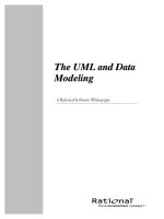
1.6 STANDING (OR STATIONARY) WAVES
The type of wave generated, for example, by plucking a string or wire stretched between
two fixed points. If the string is oriented horizontally, say, along the x-axis, the waves
moving toward the right fixed point will encounter the reflected waves moving in the
opposite direction. If the forward wave and the reflected wave have the same amplitude
at each point along the string, there will be a number of points along the string that will
have no motion. These points, in addition to the fixed anchors at the ends, correspond
to nodes where the amplitude is zero. Half-way between the nodes there will be points
where the amplitude of the wave will be maximum. The variations of amplitude are thus
a function of the distance along x. After the plucking, the resultant vibrating string will
appear to be oscillating up and down between the fixed nodes, but there will be no
motion along the length of the string—hence, the name standing or stationary wave.
Example. See Fig. 1.6.
4
ATOMIC ORBITAL THEORY
nodal points
+
−
+
−
amplitude
Figure 1.6. A standing wave; the two curves represent the time-dependent motion of a string
vibrating in the third harmonic or second overtone with four nodes.
c01.qxd 5/17/2005 5:12 PM Page 4
1.7 NODAL POINTS (PLANES)

The positions or points on a standing wave where the amplitude of the wave is zero
(Fig. 1.6). In the description of orbitals, the node represent a point or plane where a
change of sign occurs.
1.8 WAVELENGTH
λλ
The minimum distance between nearest-neighbor peaks, troughs, nodes or equiva-
lent points of the wave.
Example. The values of λ, as shown in Fig. 1.8.
1.9 FREQUENCY
νν
The number of wavelengths (or cycles) in a light wave that pass a particular point per
unit time. Time is usually measured in seconds; hence, the frequency is expressed in
s
Ϫ1
. The unit of frequency, equal to cycles per second, is called the Hertz (Hz).
Frequency is inversely proportional to wavelength; the proportionality factor is the
speed of light c (3 ϫ 10
10
cm s
Ϫ1
). Hence, ν ϭ c/λ.
Example. For light with λ equal to 300 nm (300 ϫ 10
Ϫ7
cm), the frequency ν ϭ
(3 ϫ 10
10
cm s
Ϫ1
)/(300 ϫ 10
Ϫ7

cm) ϭ 1 ϫ 10
15
s
Ϫ1
.
FREQUENCY ν
5
λ
λ
3/2 λ
1/2 λ
Figure 1.8. Determination of the wavelength λ of a wave.
c01.qxd 5/17/2005 5:12 PM Page 5
1.10 FUNDAMENTAL WAVE (OR FIRST HARMONIC)
The stationary wave with no nodal point other than the fixed ends. It is the wave
from which the frequency νЈ of all other waves in a set is generated by multiplying
the fundamental frequency ν by an integer n:
νЈϭnν (1.10)
Example. In the fundamental wave, λ/2 in Fig. 1.10, the amplitude may be consid-
ered to be oriented upward and to continuously increase from either fixed end, reach-
ing a maximum at the midpoint. In this “well-behaved” wave, the amplitude is zero
at each end and a maximum at the center.
1.11 FIRST OVERTONE (OR SECOND HARMONIC)
The stationary wave with one nodal point located at the midpoint (n ϭ 2 in the equa-
tion given in Sect. 1.10). It has half the wavelength and twice the frequency of the
first harmonic.
Example. In the first overtone (Fig. 1.11), the nodes are located at the ends and at
the point half-way between the ends, at which point the amplitude changes direction.
The two equal segments of the wave are portions of a single wave; they are not inde-
pendent. The two maximum amplitudes come at exactly equal distances from the

ends but are of opposite signs.
1.12 MOMENTUM (P)
This is the vectorial property (i.e., having both magnitude and direction) of a mov-
ing particle; it is equal to the mass m of the particle times its velocity v:
p ϭ mv (1.12)
6
ATOMIC ORBITAL THEORY
1/2 λ
Figure 1.10. The fundamental wave.
c01.qxd 5/17/2005 5:12 PM Page 6
1.13 DUALITY OF ELECTRONIC BEHAVIOR
Particles of small mass such as electrons may exhibit properties of either particles
(they have momentum) or waves (they can be defracted like light waves). A single
experiment may demonstrate either particle properties or wave properties of elec-
trons, but not both simultaneously.
1.14 DE BROGLIE RELATIONSHIP
The wavelength of a particle (an electron) is determined by the equation formulated
by Louis de Broglie (1892–1960):
λ ϭ h/p ϭ h/mv (1.14)
where h is Planck’s constant, m the mass of the particle, and v its velocity. This rela-
tionship makes it possible to relate the momentum p of the electron, a particle prop-
erty, with its wavelength λ, a wave property.
1.15 ORBITAL (ATOMIC ORBITAL)
A wave description of the size, shape, and orientation of the region in space avail-
able to an electron; each orbital has a specific energy. The position (actually the
probability amplitude) of the electron is defined by its coordinates in space, which
in Cartesian coordinates is indicated by ψ(x, y, z). ψ cannot be measured directly; it
is a mathematical tool. In terms of spherical coordinates, frequently used in calcula-
tions, the wave function is indicated by ψ(r, θ, ϕ), where r (Fig. 1.15) is the radial
distance of a point from the origin, θ is the angle between the radial line and the

ORBITAL (ATOMIC ORBITAL)
7
nodal point
λ
Figure 1.11. The first overtone (or second harmonic) of the fundamental wave.
c01.qxd 5/17/2005 5:12 PM Page 7
z-axis, and ϕ is the angle between the x-axis and the projection of the radial line on
the xy-plane. The relationship between the two coordinate systems is shown in
Fig. 1.15. An orbital centered on a single atom (an atomic orbital) is frequently
denoted as φ (phi) rather than ψ (psi) to distinguish it from an orbital centered on
more than one atom (a molecular orbital) that is almost always designated ψ.
The projection of r on the z-axis is z ϭ OB, and OBA is a right angle. Hence,
cos θ ϭ z /r, and thus, z ϭ r cos θ. Cos ϕ ϭ x/OC, but OC ϭ AB ϭ r sin θ. Hence, x ϭ
r sin θ cos ϕ. Similarly, sin ϕ ϭ y/AB; therefore, y ϭ AB sin ϕ ϭ r sin θ sin ϕ.
Accordingly, a point (x, y, z) in Cartesian coordinates is transformed to the spherical
coordinate system by the following relationships:
z ϭ r cos θ
y ϭ r sin θ sin ϕ
x ϭ r sin θ cos ϕ
1.16 WAVE FUNCTION
In quantum mechanics, the wave function is synonymous with an orbital.
8
ATOMIC ORBITAL THEORY
Z
x
y
z
r
θ
φ

φ
θ
Origin (0)
volume element
of space (dτ)
B
A
Y
X
C
Figure 1.15. The relationship between Cartesian and polar coordinate systems.
c01.qxd 5/17/2005 5:12 PM Page 8
1.17 WAVE EQUATION IN ONE DIMENSION
The mathematical description of an orbital involving the amplitude behavior of a
wave. In the case of a one-dimensional standing wave, this is a second-order differ-
ential equation with respect to the amplitude:
d
2
f(x)/dx
2
ϩ (4π
2
/λ
2
) f (x) ϭ 0 (1.17)
where λ is the wavelength and the amplitude function is f(x).
1.18 WAVE EQUATION IN THREE DIMENSIONS
The function f (x, y, z) for the wave equation in three dimensions, analogous to f(x),
which describes the amplitude behavior of the one-dimensional wave. Thus, f (x, y, z)
satisfies the equation

Ѩ
2
f(x)/Ѩx
2
ϩѨ
2
f(y)/Ѩ y
2
ϩѨ
2
f (z)/Ѩz
2
ϩ (4π
2
/λ
2
) f(x, y, z) ϭ 0 (1.18)
In the expression Ѩ
2
f(x)/Ѩx
2
, the portion Ѩ
2
/Ѩx
2
is an operator that says “partially dif-
ferentiate twice with respect to x that which follows.”
1.19 LAPLACIAN OPERATOR
The sum of the second-order differential operators with respect to the three Cartesian
coordinates in Eq. 1.18 is called the Laplacian operator (after Pierre S. Laplace,

1749–1827), and it is denoted as ∇
2
(del squared):
∇
2
ϭѨ
2
/Ѩx
2
ϩѨ
2
/Ѩy
2
ϩѨ
2
/Ѩz
2
(1.19a)
which then simplifies Eq. 1.18 to
∇
2
f(x, y, z) ϩ (4π
2
/λ
2
) f(x, y, z) ϭ 0 (1.19b)
1.20 PROBABILITY INTERPRETATION OF THE WAVE FUNCTION
The wave function (or orbital) ψ(r), because it is related to the amplitude of a wave
that determines the location of the electron, can have either negative or positive val-
ues. However, a probability, by definition, must always be positive, and in the pres-

ent case this can be achieved by squaring the amplitude. Accordingly, the probability
of finding an electron in a specific volume element of space d
τ
at a distance r from
the nucleus is ψ(r)
2
dτ. Although ψ, the orbital, has mathematical significance (in
PROBABILITY INTERPRETATION OF THE WAVE FUNCTION
9
c01.qxd 5/17/2005 5:12 PM Page 9
that it can have negative and positive values), ψ
2
has physical significance and is
always positive.
1.21 SCHRÖDINGER EQUATION
This is a differential equation, formulated by Erwin Schrödinger (1887–1961),
whose solution is the wave function for the system under consideration. This equa-
tion takes the same form as an equation for a standing wave. It is from this form of
the equation that the term wave mechanics is derived. The similarity of the
Schrödinger equation to a wave equation (Sect. 1.18) is demonstrated by first sub-
stituting the de Broglie equation (1.14) into Eq. 1.19b and replacing f by φ:
∇
2
φ ϩ (4π
2
m
2
v
2
/h

2
)φ ϭ 0 (1.21a)
To incorporate the total energy E of an electron into this equation, use is made of the
fact that the total energy is the sum of the potential energy V, plus the kinetic energy,
1/2 mv
2
,or
v
2
ϭ 2(E Ϫ V )/m (1.21b)
Substituting Eq. 1.21b into Eq. 1.21a gives Eq. 1.21c:
∇
2
φ ϩ (8π
2
m/h
2
)(E Ϫ V )φ ϭ 0 (1.21c)
which is the Schrödinger equation.
1.22 EIGENFUNCTION
This is a hybrid German-English word that in English might be translated as “char-
acteristic function”; it is an acceptable solution of the wave equation, which can be
an orbital. There are certain conditions that must be fulfilled to obtain “acceptable”
solutions of the wave equation, Eq. 1.17 [e.g., f(x) must be zero at each end, as in the
case of the vibrating string fixed at both ends; this is the so-called boundary condi-
tion]. In general, whenever some mathematical operation is done on a function and
the same function is regenerated multiplied by a constant, the function is an eigen-
function, and the constant is an eigenvalue. Thus, wave Eq. 1.17 may be written as
d
2

f(x)/dx
2
ϭϪ(4π
2
/λ
2
) f(x) (1.22)
This equation is an eigenvalue equation of the form:
(Operator) (eigenfunction) ϭ (eigenvalue) (eigenfunction)
10
ATOMIC ORBITAL THEORY
c01.qxd 5/17/2005 5:12 PM Page 10
where the operator is (d
2
/dx
2
), the eigenfunction is f(x), and the eigenvalue is (4π
2
/λ
2
).
Generally, it is implied that wave functions, hence orbitals, are eigenfunctions.
1.23 EIGENVALUES
The values of λ calculated from the wave equation, Eq. 1.17. If the eigenfunction is
an orbital, then the eigenvalue is related to the orbital energy.
1.24 THE SCHRÖDINGER EQUATION FOR THE HYDROGEN ATOM
An (eigenvalue) equation, the solutions of which in spherical coordinates are
φ(r, θ, ϕ) ϭ R(r) Θ(θ) Φ(ϕ) (1.24)
The eigenfunctions φ, also called orbitals, are functions of the three variables shown,
where r is the distance of a point from the origin, and θ and ϕ are the two angles

required to locate the point (see Fig. 1.15). For some purposes, the spatial or radial
part and the angular part of the Schrödinger equation are separated and treated inde-
pendently. Associated with each eigenfunction (orbital) is an eigenvalue (orbital
energy). An exact solution of the Schrödinger equation is possible only for the
hydrogen atom, or any one-electron system. In many-electron systems wave func-
tions are generally approximated as products of modified one-electron functions
(orbitals). Each solution of the Schrödinger equation may be distinguished by a set
of three quantum numbers, n, l, and m, that arise from the boundary conditions.
1.25 PRINCIPAL QUANTUM NUMBER n
An integer 1, 2, 3,...,that governs the size of the orbital (wave function) and deter-
mines the energy of the orbital. The value of n corresponds to the number of the shell
in the Bohr atomic theory and the larger the n, the higher the energy of the orbital
and the farther it extends from the nucleus.
1.26 AZIMUTHAL (ANGULAR MOMENTUM)
QUANTUM NUMBER l
The quantum number with values of l ϭ 0,1,2,...,(n Ϫ 1) that determines the shape
of the orbital. The value of l implies particular angular momenta of the electron
resulting from the shape of the orbital. Orbitals with the azimuthal quantum numbers
l ϭ 0, 1, 2, and 3 are called s, p, d, and f orbitals, respectively. These orbital desig-
nations are taken from atomic spectroscopy where the words “sharp”, “principal”,
“diffuse”, and “fundamental” describe lines in atomic spectra. This quantum num-
ber does not enter into the expression for the energy of an orbital. However, when
AZIMUTHAL (ANGULAR MOMENTUM) QUANTUM NUMBER l
11
c01.qxd 5/17/2005 5:12 PM Page 11
electrons are placed in orbitals, the energy of the orbitals (and hence the energy of
the electrons in them) is affected so that orbitals with the same principal quantum
number n may vary in energy.
Example. An electron in an orbital with a principal quantum number of n ϭ 2 can
take on l values of 0 and 1, corresponding to 2s and 2p orbitals, respectively. Although

these orbitals have the same principal quantum number and, therefore, the same
energy when calculated for the single electron hydrogen atom, for the many-electron
atoms, where electron–electron interactions become important, the 2p orbitals are
higher in energy than the 2s orbitals.
1.27 MAGNETIC QUANTUM NUMBER m
l
This is the quantum number having values of the azimuthal quantum number from
ϩl to Ϫl that determines the orientation in space of the orbital angular momentum;
it is represented by m
l
.
Example. When n ϭ 2 and l ϭ 1 (the p orbitals), m
l
may thus have values of ϩ1, 0,
Ϫ1, corresponding to three 2p orbitals (see Sect. 1.35). When n ϭ 3 and l ϭ 2, m
l
has
the values of ϩ2, ϩ1, 0, Ϫ1, Ϫ2 that describe the five 3d orbitals (see Sect. 1.36).
1.28 DEGENERATE ORBITALS
Orbitals having equal energies, for example, the three 2p orbitals.
1.29 ELECTRON SPIN QUANTUM NUMBER m
s
This is a measure of the intrinsic angular momentum of the electron due to the fact
that the electron itself is spinning; it is usually designated by m
s
and may only have
the value of 1/2 or Ϫ1/2.
1.30 s ORBITALS
Spherically symmetrical orbitals; that is, φ is a function of R(r) only. For s orbitals,
l ϭ 0 and, therefore, electrons in such orbitals have an orbital magnetic quantum

number m
l
equal to zero.
1.31 1s ORBITAL
The lowest-energy orbital of any atom, characterized by n ϭ 1, l ϭ m
l
ϭ 0. It corre-
sponds to the fundamental wave and is characterized by spherical symmetry and no
12
ATOMIC ORBITAL THEORY
c01.qxd 5/17/2005 5:12 PM Page 12
nodes. It is represented by a projection of a sphere (a circle) surrounding the nucleus,
within which there is a specified probability of finding the electron.
Example. The numerical probability of finding the hydrogen electron within spheres
of various radii from the nucleus is shown in Fig. 1.31a. The circles represent con-
tours of probability on a plane that bisects the sphere. If the contour circle of 0.95
probability is chosen, the electron is 19 times as likely to be inside the correspon-
ding sphere with a radius of 1.7 Å as it is to be outside that sphere. The circle that is
usually drawn, Fig. 1.31b, to represent the 1s orbital is meant to imply that there is
a high, but unspecified, probability of finding the electron in a sphere, of which the
circle is a cross-sectional cut or projection.
1.32 2s ORBITAL
The spherically symmetrical orbital having one spherical nodal surface, that is, a sur-
face on which the probability of finding an electron is zero. Electrons in this orbital
have the principal quantum number n ϭ 2, but have no angular momentum, that is,
l ϭ 0, m
l
= 0.
Example. Figure 1.32 shows the probability distribution of the 2s electron as a cross
section of the spherical 2s orbital. The 2s orbital is usually drawn as a simple circle of

arbitrary diameter, and in the absence of a drawing for the 1s orbital for comparison,
2s ORBITAL
13
1.2
1.6
2.0
0.95
0.9
0.8
0.7
0.5
0.4 0.8
0.3
0.1
(a)
(b)
probability
radius (Å)
Figure 1.31. (a) The probability contours and radii for the hydrogen atom, the probability at
the nucleus is zero. (b) Representation of the 1s orbital.
c01.qxd 5/17/2005 5:12 PM Page 13
the two would be indistinguishable despite the larger size of the 2s orbital and the fact
that there is a nodal surface within the 2s sphere that is not shown in the simple circu-
lar representation.
1.33 p ORBITALS
These are orbitals with an angular momentum l equal to 1; for each value of the prin-
cipal quantum number n (except for n ϭ 1), there will be three p orbitals correspon-
ding to m
l
ϭϩ1, 0, Ϫ1. In a useful convention, these three orbitals, which are

mutually perpendicular to each other, are oriented along the three Cartesian coordi-
nate axes and are therefore designated as p
x
, p
y
,and p
z
. They are characterized by
having one nodal plane.
1.34 NODAL PLANE OR SURFACE
A plane or surface associated with an orbital that defines the locus of points for which
the probability of finding an electron is zero. It has the same meaning in three dimen-
sions that the nodal point has in the two-dimensional standing wave (see Sect. 1.7)
and is associated with a change in sign of the wave function.
14
ATOMIC ORBITAL THEORY
nodal
contour region
95% contour line
Figure 1.32. Probability distribution ψ
2
for the 2s orbital.
c01.qxd 5/17/2005 5:12 PM Page 14
1.35 2p ORBITALS
The set of three degenerate (equal energy) atomic orbitals having the principal quan-
tum number (n) of 2, an azimuthal quantum number (l) of 1, and magnetic quantum
numbers (m
l
) of ϩ1, 0, or Ϫ1. Each of these orbitals has a nodal plane.
Example. The 2p orbitals are usually depicted so as to emphasize their angular

dependence, that is, R(r) is assumed constant, and hence are drawn for conven-
ience as a planar cross section through a three-dimensional representation of
Θ(θ)Φ(ϕ). The planar cross section of the 2p
z
orbital, ϕ ϭ 0, then becomes a pair
of circles touching at the origin (Fig. 1.35a). In this figure the wave function
(without proof ) is φ ϭ Θ(θ) ϭ (͙6
ෆ
/2)cos θ. Since cos θ, in the region
90° Ͻ θ Ͻ 270°, is negative, the top circle is positive and the bottom circle nega-
tive. However, the physically significant property of an orbital φ is its square, φ
2
;
the plot of φ
2
ϭ Θ
2
(θ) ϭ 3/2 cos
2
θ for the p
z
orbital is shown in Fig. 1.35b, which
represents the volume of space in which there is a high probability of finding the
electron associated with the p
z
orbital. The shape of this orbital is the familiar
elongated dumbbell with both lobes having a positive sign. In most common
drawings of the p orbitals, the shape of φ
2
, the physically significant function, is

retained, but the plus and minus signs are placed in the lobes to emphasize the
nodal property, (Fig. 1.35c). If the function R(r) is included, the oval-shaped con-
tour representation that results is shown in Fig. 1.35d, where φ
2
( p
z
) is shown as a
cut in the yz-plane.
2p ORBITALS
15
(d)
y
z
0.50
1.00
1.50
90°
−
180°
270°
0°
units of
Bohr radii
+
(a)
(b)
(c)
p
x
p

z
p
y
+
+
+
−
−
−
Figure 1.35. (a) The angular dependence of the p
z
orbital; (b) the square of (a); (c) the com-
mon depiction of the three 2p orbitals; and (d) contour diagram including the radial depend-
ence of φ.
c01.qxd 5/17/2005 5:12 PM Page 15
1.36 d ORBITALS
Orbitals having an angular momentum l equal to 2 and, therefore, magnetic quantum
numbers, (m
l
) of ϩ2, ϩ1, 0, Ϫ1, Ϫ2. These five magnetic quantum numbers
describe the five degenerate d orbitals. In the Cartesian coordinate system, these
orbitals are designated as d
z
2
, d
x
2
᎐ y
2
,

d
xy
, d
xz
, and d
yz
; the last four of these d orbitals
are characterized by two nodal planes, while the d
z
2
has surfaces of revolution.
Example. The five d orbitals are depicted in Fig. 1.36. The d
z
2
orbital that by con-
vention is the sum of d
z
2
᎐ x
2
and d
z
2
᎐ y
2
and, hence, really d
2 z
2
᎐x
2

᎐ y
2
is strongly directed
along the z-axis with a negative “doughnut” in the xy-plane. The d
x
2
᎐ y
2
orbital has
lobes pointed along the x- and y-axes, while the d
xy
, d
xz
, and d
yz
orbitals have lobes that
are pointed half-way between the axes and in the planes designated by the subscripts.
1.37 f ORBITALS
Orbitals having an angular momentum l equal to 3 and, therefore, magnetic quantum
numbers, m
l
of ϩ3, ϩ2, ϩ1, 0, Ϫ1, Ϫ2, Ϫ3. These seven magnetic quantum numbers
16
ATOMIC ORBITAL THEORY
y
z
x
d
z
2

d
x
2
−y
2
d
yz
d
xy
d
xz
Figure 1.36. The five d orbitals. The shaded and unshaded areas represent lobes of different
signs.
c01.qxd 5/17/2005 5:12 PM Page 16
describe the seven degenerate f orbitals. The f orbitals are characterized by three nodal
planes. They become important in the chemistry of inner transition metals (Sect. 1.44).
1.38 ATOMIC ORBITALS FOR MANY-ELECTRON ATOMS
Modified hydrogenlike orbitals that are used to describe the electron distribution in
many-electron atoms. The names of the orbitals, s, p, and so on, are taken from the
corresponding hydrogen orbitals. The presence of more than one electron in a many-
electron atom can break the degeneracy of orbitals with the same n value. Thus, the
2p orbitals are higher in energy than the 2s orbitals when electrons are present in
them. For a given n, the orbital energies increase in the order s Ͻ p Ͻ d Ͻ f Ͻ ....
1.39 PAULI EXCLUSION PRINCIPLE
According to this principle, as formulated by Wolfgang Pauli (1900–1958), a maxi-
mum of two electrons can occupy an orbital, and then, only if the spins of the elec-
trons are opposite (paired), that is, if one electron has m
s
ϭϩ1/2, the other must have
m

s
ϭϪ1/2. Stated alternatively, no two electrons in the same atom can have the same
values of n, l, m
l
, and m
s
.
1.40 HUND’S RULE
According to this rule, as formulated by Friedrich Hund (1896–1997), a single elec-
tron is placed in all orbitals of equal energy (degenerate orbitals) before a second elec-
tron is placed in any one of the degenerate set. Furthermore, each of these electrons in
the degenerate orbitals has the same (unpaired) spin. This arrangement means that
these electrons repel each other as little as possible because any particular electron is
prohibited from entering the orbital space of any other electron in the degenerate set.
1.41 AUFBAU (GER. BUILDING UP) PRINCIPLE
The building up of the electronic structure of the atoms in the Periodic Table. Orbitals
are indicated in order of increasing energy and the electrons of the atom in question
are placed in the unfilled orbital of lowest energy, filling this orbital before proceeding
to place electrons in the next higher-energy orbital. The sequential placement of elec-
trons must also be consistent with the Pauli exclusion principle and Hund’s rule.
Example. The placement of electrons in the orbitals of the nitrogen atom (atomic
number of 7) is shown in Fig. 1.41. Note that the 2p orbitals are higher in energy
than the 2s orbital and that each p orbital in the degenerate 2p set has a single elec-
tron of the same spin as the others in this set.
AUFBAU (G. BUILDING UP) PRINCIPLE
17
c01.qxd 5/17/2005 5:12 PM Page 17
1.42 ELECTRONIC CONFIGURATION
The orbital occupation of the electrons of an atom written in a notation that consists
of listing the principal quantum number, followed by the azimuthal quantum num-

ber designation (s, p, d, f ), followed in each case by a superscript indicating the
number of electrons in the particular orbitals. The listing is given in the order of
increasing energy of the orbitals.
Example. The total number of electrons to be placed in orbitals is equal to the atomic
number of the atom, which is also equal to the number of protons in the nucleus of the
atom. The electronic configuration of the nitrogen atom, atomic number 7 (Fig. 1.41),
is 1s
2
2s
2
2p
3
; for Ne, atomic number 10, it is 1s
2
2s
2
2p
6
; for Ar, atomic number 18, it
is 1s
2
2s
2
2p
6
3s
2
3p
6
; and for Sc, atomic number 21, it is [Ar]4s

2
3d
1
,where [Ar] repre-
sents the rare gas, 18-electron electronic configuration of Ar in which all s and p
orbitals with n ϭ 1 to 3, are filled with electrons. The energies of orbitals are approxi-
mately as follows: 1s Ͻ2s Ͻ2p Ͻ3s Ͻ3p Ͻ 4s ≈3d Ͻ 4p Ͻ 5s ≈ 4d.
1.43 SHELL DESIGNATION
The letters K, L, M, N, and O are used to designate the principal quantum number n.
Example. The 1s orbital which has the lowest principal quantum number, n ϭ 1, is
designated the K shell; the shell when n ϭ 2 is the L shell, made up of the 2s,2p
x
,2p
y
,
and 2p
z
orbitals; and the shell when n ϭ 3 is the M shell consisting of the 3s, the three
3p orbitals, and the five 3d orbitals. Although the origin of the use of the letters K, L,
M, and so on, for shell designation is not clearly documented, it has been suggested
that these letters were abstracted from the name of physicist Charles Barkla (1877–
1944, who received the Nobel Prize, in 1917). He along with collaborators had noted
that two rays were characteristically emitted from the inner shells of an element after
18
ATOMIC ORBITAL THEORY
1s
2s
2p
Figure 1.41. The placement of electrons in the orbitals of the nitrogen atom.
c01.qxd 5/17/2005 5:12 PM Page 18