Solution manual engineering economic analysis 9th edition ch02

Chapter 2: Engineering Costs and Cost Estimating
2-1
This is an example of a ‘sunk cost.’ The $4,000 is a past cost and should not be allowed to alter
a subsequent decision unless there is some real or perceived effect. Since either home is really
an individual plan selected by the homeowner, each should be judged in terms of value to the
homeowner vs. the cost. On this basis the stock plan house appears to be the preferred
alternative.
2-2
Unit Manufacturing Cost
(a) Daytime Shift = ($2,000,000 + $9,109,000)/23,000 = $483/unit
(b) Two Shifts
= [($2,400,000 + (1 + 1.25) ($9,109,000)]/46,000
= $497.72/unit
Second shift increases unit cost.
2-3
(a) Monthly Bill:
50 x 30
Total

= 1,500 kWh @ $0.086
= $129.00
= 1,300 kWh @ $0.066
= $85.80
= 2,800 kWh
= $214.80

Average Cost = $214.80/2,800
= $129.00
Marginal Cost (cost for the next kWh)
= $0.066 because the 2,801st kWh is in the
2nd bracket of the cost structure.

($0.066 for 1,501-to-3,000 kWh)
(b) Incremental cost of an additional 1,200 kWh/month:
200 kWh x $0.066
= $13.20
1,000 kWh x $0.040 = $40.00
1,200 kWh
$53.20
(c) New equipment:
Assuming the basic conditions are 30 HP and 2,800 kWh/month
Monthly bill with new equipment installed:
50 x 40
= 2,000 kWh at $0.086
= $172.00
900 kWh at $0.066 = $59.40
2,900 kWh
$231.40
Incremental cost of energy = $231.40 - $214.80 = $16.60
Incremental unit cost = $16.60/100
= $0.1660/kWh


2-4
x = no. of maps dispensed per year
(a)
(b)
(c)
(d)
(e)

Fixed Cost (I) = $1,000

Fixed Cost (II) = $5,000
Variable Costs (I)
= 0.800
Variable Costs (II)
= 0.160
Set Total Cost (I)
= Total Cost (II)
$1,000 + 0.90 x
= $5,000 + 0.10 x
thus x = 5,000 maps dispensed per year.
The student can visually verify this from the figure.
(f) System I is recommended if the annual need for maps is <5,000
(g) System II is recommended if the annual need for maps is >5,000
(h) Average Cost @ 3,000 maps:
TC(I) = (0.9) (3.0) + 1.0
= 3.7/3.0
= $1.23 per map
TC(II) = (0.1) (3.0) + 5.0
= 5.3/3.0
= $1.77 per map
Marginal Cost is the variable cost for each alternative, thus:
Marginal Cost (I)
= $0.90 per map
Marginal Cost (II)
= $0.10 per map
2-5
C = $3,000,000 - $18,000Q + $75Q2
Where C = Total cost per year
Q = Number of units produced per year
Set the first derivative equal to zero and solve for Q.

dC/dQ = -$18,000 + $150Q = 0
Q = $18,000/$150 = 120
Therefore total cost is a minimum at Q equal to 120. This indicates that production below
120 units per year is most undesirable, as it costs more to produce 110 units than to
produce 120 units.
Check the sign of the second derivative:
d2C/dQ2 = +$150
The + indicates the curve is concave upward, ensuring that Q = 120 is the point of a
minimum.
Average unit cost at Q = 120/year:
= [$3,000,000 - $18,000 (120) + $75 (120)2]/120

= $16,000

Average unit cost at Q = 110/year:
= [$3,000,000 - $18,000 (110) + $75 (120)2]/110

= $17,523


One must note, of course, that 120 units per year is not necessarily the optimal level of
production. Economists would remind us that the optimum point is where Marginal Cost =
Marginal Revenue, and Marginal Cost is increasing. Since we do not know the Selling
Price, we cannot know Marginal Revenue, and hence we cannot compute the optimum level
of output.
We can say, however, that if the firm is profitable at the 110 units/year level, then it will be
much more profitable at levels greater than 120 units.
2-6
x = number of campers
(a) Total Cost

= Fixed Cost + Variable Cost
= $48,000 + $80 (12) x
Total Revenue = $120 (12) x
(b) Break-even when Total Cost = Total Revenue
$48,000 + $960 x
= $1,440 x
$4,800
= $480 x
x = 100 campers to break-even
(c) capacity is 200 campers
80% of capacity is 160 campers
@ 160 campers x = 160
Total Cost
= $48,000 + $80 (12) (160) = $201,600
Total Revenue = $120 (12) (160)
= $230,400
Profit = Revenue – Cost
= $230,400 - $201,600
= $28,800
2-7
(a) x = number of visitors per year
Break-even when: Total Costs (Tugger) = Total Costs (Buzzer)
$10,000 + $2.5 x = $4,000 + $4.00 x
x = 400 visitors is the break-even quantity
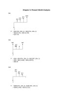
(b) See the figure below:
X
0
4,000
8,000

Y1 (Tug)
10,000
20,000
30,000

Y2 (Buzz)
4,000
20,000
36,000


Y1 (Tug)
Y2 (Buzz)

$40,000

Y2 = 4,000 + 4x
$30,000

Y1 = 10,000 + 2.5x

$20,000
$10,000

Tug
Preferred

0

2,000

Buzz
Preferred

4,000
6,000
Visitors per year

8,000

2-8
x = annual production
(a) Total Revenue = ($200,000/1,000) x = $200 x
(b) Total Cost

= $100,000 + ($100,000/1,000)x

= $100,000 + $100 x

(c) Set Total Cost = Total Revenue
$200 x = $100,000 + $100 x
x = 1,000 units per year
The student can visually verify this from the figure.
(d) Total Revenue = $200 (1,500)
= $300,000
Total Cost
= $100,000 + $100 (150
= $250,000
Profit

= $300,000 - $250,000
= $50,000

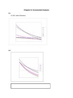
2-9
x = annual production
Let’s look at the graphical solution first, where the cost equations are:
Total Cost (A) = $20 x + $100,000
Total Cost (B) = $5 x + $200,000
Total Cost (C) = $7.5 x + $150,000
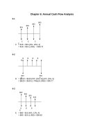
[See graph below]


Quatro Hermanas wants to minimize costs over all ranges of x. From the graph we see that
there are three break-even points: A & B, B & C, and A & C. Only A & C and B & C are
necessary to determine the minimum cost alternative over x. Mathematically the break-even
points are:
A & C: $20 x + $100,000
B & C: $5 x + $200,000

= $7.5 x + $150,000
= $8.5 x + $150,000

x = 4,000
x = 20,000

Thus our recommendation is, if:
0 < x < 4,000
choose Alternative A
4,000 < x < 20,000
choose Alternative C

20,000 < x 30,000 choose Alternative B
X
0
10
20
30

A
100
300
500
700

B
200
250
300
350

C
150
225
300
375

A
B
C

$800

YA = 100,000 + 20x
$600
YC = 150,000 + 7.5x

$400

YB = 200,000 + 5x

$200
A
Best
0

5

B Preferred
BE = 25,000

C Preferred
BE = 100,000

10 15
20 25
30
Production Volume (1,000 units)

2-10
x

= annual production rate

(a) There are three break-even points for total costs for the three alternatives
A & B: $20.5 x + $100,000 = $10.5 x + $350,000
x = 25,000
B & C: $10.5 x + $350,000 = $8 x + $600,000
x = 100,000


A & C: $20 x + $100,000
x = 40,000

= $8 x + $600,000

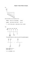
We want to minimize costs over the range of x, thus the A & C break-even point is not of
interest. Sneaking a peak at the figure below we see that if:
0 < x < 25,000
choose A
25,000 < x < 80,000
choose B
80,000 < x < 100,000
choose C
(b) See graph below for Solution:
X
0
50
100
150

A

100
1,125
2,150
3,175

B
350
875
1,400
1,925

C
600
1,000
1,400
1,800
A
B
C
YA = 100,000 + 20.5x

$2,500

YB = 350,000 + 10.5x

$2,000

YC = 600,000 + 8x

$1,500

$1,000
$500

A
0

B Preferred
BE = 25,000

C Preferred
BE = 100,000

50
100
150
Production Volume (1,000 units)

2-11
x = annual production volume (demand) = D
(a) Total Cost
= $10,875 + $20 x
Total Revenue = (price per unit) (number sold)
= ($0.25 D + $250) D and if D = x
= -$0.25 x2 + $250 x
(b) Set Total Cost = Total Revenue
$10,875 + $20 x
= -$0.25 x2 + $250 x
2
-$0.25 x + $230 x - $10,875 = 0
This polynomial of degree 2 can be solved using the quadratic formula:

There will be two solutions:
x = (-b + (b2 – 4ac)1/2)/2a = (-$230 + $205)/-0.50
Thus x = 870 and x = 50. There are two levels of x where TC = TR.
(c) To maximize Total Revenue we will take the first derivative of the Total Revenue
equation, set it equal to zero, and solve for x:
TR = -$0.25 x2 + $250 x
dTR/dx = -$0.50 x + $250 = 0
x = 500 is where we realize maximum revenue
(d) Profit is revenue – cost, thus let’s find the profit equation and do the same process as in
part (c).
Total Profit = (-$0.25 x2 + $250 x) – ($10,875 + $20 x)
= -$0.25 x2 + $230 x - $10,875
dTP/dx = -$0.50 x + $230 = 0
x = 460 is where we realize our maximum profit
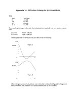
(e) See the figure below. Your answers to (a) – (d) should make sense now.
X
0
250
500
750
1,000

Total Cost
$10,875
$15,875
$20,875
$25,875
$30,875

Total Revenue
$0
$46,875
$62,500
$46,875
$0

Total Cost
Total Revenue

TR = 250 x – 0.25x2

$60,000
$40,000

Max
Profit

Max
Revenue

BE = 870
TC = 10,875 + 20x

$20,000
BE = 50
0

200

400
600
Annual Production

800

1,000


2-12
x = units/year
By hand
$1.40 x
x

= Painting Machine
= $15,000/4 + $0.20
= $5,000/1.20 = $4,167 units

2-13
x = annual production units
Total Cost to Company A
= Total Cost to Company B
$15,000 + $0.002 x = $5,000 + $0.05 x
x = $10,000/$0.048
= 208,330 units

2-14
(a)

$2,500
$2,000
Total
Cost &
Income

TC = 1,000 + 10S

$1,500
$1,000

Breakeven

Total Income

$500

0

20

Profit = S ($100 – S) - $1,000 - $10 S

40
60
Sales Volume (S)

80

= -S2 + $90 S - $1,000

(b) For break-even, set Profit = 0
-S2 + $90S - $1,000 = $0
S
= (-b + (b2 – 4ac)1/2)/2a = (-$90 + ($902 – (4) (-1) (-1,000))1/2)/-2
= 12.98, 77.02
(c) For maximum profit
dP/dS = -$2S + $90 = $0
S = 45 units
Answers: Break-even at 14 and 77 units. Maximum profit at 45 units.

100


Alternative Solution: Trial & Error
Price

Sales Volume

$20
$23
$30
$50
$55
$60
$80
$87
$90

80

77
70
50
45
40
20
13
10

Total
Income
$1,600
$1,771
$2,100
$2,500
$2,475
$2,400
$1,600
$1,131
$900

Total Cost

Profit

$1,800
$1,770
$1,700
$1,500
$1,450

$1,400
$1,200
$1,130
$1,100

-$200
$0 (Break-even)
$400
$1,000
$1,025
$1,000
$400
$0 (Break-even)
-$200

2-15
In this situation the owners would have both recurring costs (repeating costs per some time
period) as well as non-recurring costs (one time costs). Below is a list of possible recurring
and non-recurring costs. Students may develop others.
Recurring Costs
Non-recurring costs
- Annual inspection costs
- Initial construction costs
- Annual costs of permits
- Legal costs to establish rental
- Carpet replacement costs
- Drafting of rental contracts
- Internal/external paint costs
- Demolition costs
- Monthly trash removal costs

- Monthly utilities costs
- Annual costs for accounting/legal
- Appliance replacements
- Alarms, detectors, etc. costs
- Remodeling costs (bath, bedroom)
- Durable goods replacements
(furnace, air-conditioner, etc.)

2-16
A cash cost is a cost in which there is a cash flow exchange between or among parties. This
term derives from ‘cash’ being given from one entity to another (persons, banks, divisions,
etc.). With today’s electronic banking capabilities cash costs may or may not involve ‘cash.’
‘Book costs’ are costs that do not involve an exchange of ‘cash’, rather, they are only
represented on the accounting books of the firm. Book costs are not represented as beforetax cash flows.
Engineering economic analyses can involve both cash and book costs. Cash costs are the
before-tax cash flows usually estimated for a project (such as initial costs, annual costs, and
retirement costs) as well as costs due to financing (payments on principal and interest debt)


and taxes. Cash costs are important in such cases. For the engineering economist the
primary book cost that is of concern is equipment depreciation, which is accounted for in
after-tax analyses.

2-17
Here the student may develop several different thoughts as it relates to life-cycle costs. By
life-cycle costs the authors are referring to any cost associated with a product, good, or
service from the time it is conceived, designed, constructed, implemented, delivered,
supported and retired. Firms should be aware of and account for all activities and liabilities
associated with a product through its entire life-cycle. These costs and liabilities represent
real cash flows for the firm  either at the time or some time in the future.

2-18
Figure 2-4 illustrates the difference between ‘dollars spent’ and ‘dollars committed’ over the
life cycle of a project. The key point being that most costs are committed early in the life
cycle, although they are not realized until later in the project. The implication of this effect is
that if the firm wants to maximize value-per-dollar spent, the time to make important design
decisions (and to account for all life cycle effects) is early in the life cycle. Figure 2-5
demonstrates ‘ease of making design changes’ and ‘cost of design changes’ over a project’s
life cycle. The point of this comparison is that the early stages of the design cycle are the
easiest and least costly periods to make changes. Both figures represent important effects
for firms.
In summary, firms benefit from spending time, money and effort early in the life cycle.
Effects resulting from early decisions impact the overall life cycle cost (and quality) of the
product, good, or service. An integrated, cross-functional, enterprise-wide approach to
product design serves the modern firm well.

2-19
In this chapter, the authors list the following three factors as creating difficulties in making
cost estimates: One-of-a-Kind Estimates, Time and Effort Available, and Estimator
Expertise. Each of these factors could influence the estimate, or the estimating process, in
different scenarios in different firms. One-of-a-kind estimating is a particularly challenging
aspect for firms with little corporate-knowledge or suitable experience in an industry.
Estimates, bids and budgets could potentially vary greatly in such circumstances. This is
perhaps the most difficult of the factors to overcome. Time and effort can be influenced, as
can estimator expertise. One-of-a-kind estimates pose perhaps the greatest challenge.

2-20
Total Cost = Phone unit cost + Line cost + One Time Cost
= ($100/2) 125 + $7,500 (100) + $10,000
= $766,250

Cost to State

= $766,250 (1.35)

= $1,034,438

2-21
Cost (total) = Cost (paint) + Cost (labour) + Cost (fixed)
Number of Cans needed = (6,000/300) (2)

= 40 cans

Cost (paint)

= (10 cans) $15
= $150.00
= (15 cans) $10
= $150.00
= (15 cans) $7.50
= $112.50
Total
= $412.50
Cost (labour) = (5 painters) (10 hrs/day) (4.5 days/job) ($8.75/hr)
= $1,968.75
Cost (total)
= $412.50 + $1,968.75 + $200
= $2,581.25

2-22
(a) Unit Cost = $150,000/2,000 = $75/ft2
(bi) If all items change proportionately, then:
Total Cost
= ($75/ft2) (4,000 ft2) = $300,000
(bii) For items that change proportionately to the size increase we multiply by: 4,000/2,000
= 2.0 all the others stay the same.
[See table below]
Cost
item
1
2
3
4
5
6
7
8

2,000 ft2 House Cost

Increase

($150,000) (0.08) = $12,000
($150,000) (0.15) = $22,500
($150,000) (0.13) = $19,500
($150,000) (0.12) = $18,000
($150,000) (0.13) = $19,500
($150,000) (0.20) = $30,000
($150,000) (0.12) = $18,000

($150,000) (0.17) = $25,500

x1
x1
x2
x2
x2
x2
x2
x2
Total Cost

4,000 ft2
House Cost
$12,000
$22,500
$39,000
$36,000
$39,000
$60,000
$36,000
$51,000
= $295,500

2-23
(a) Unit Profit

= $410 (0.30) = $123 or
= Unit Sales Price – Unit Cost
= $410 (1.3) - $410 = $533 - $410 = $123

(b) Overall Batch Cost = $410 (10,000)
= $4,100,000


(c) Of the 10,000 batch:
1. (10,000) (0.01)
2. (10,000 – 100) (0.03)
3. (9,900 – 297) (0.02)
Total
Overall Batch Profit

= 100 are scrapped in mfg.
= 297 of finished product go unsold
= 192 of sold product are not returned
= 589 of original batch are not sold for profit

= (10,000 – 589) $123

= $1,157,553

(d) Unit Cost
= 112 ($0.50) + $85 + $213 = $354
Batch Cost with Contract
= 10,000 ($354)
= $3,540,000
Difference in Batch Cost:
= BC without contract- BC with contract
= $4,100,000 - $3,540,000
= $560,000
SungSam can afford to pay up to $560,000 for the contract.

2-24
CA/CB
= IA/IB
C50 YEARS AGO/CTODAY = AFCI50 YEARS AGO/AFCITODAY
CTODAY
= ($2,050/112) (55) = $1,007
2-25
ITODAY
CLAST YEAR

= (72/12) (100)
= 600
= (525/600) (72)
= $63

2-26
Equipment
Varnish Bath
Power Scraper
Paint Booth

Cost of New
Equipment minus
(75/50)0.80 (3,500) =
$4,841
(1.5/0.75)0.22 (250) =
$291
(12/3)0.6 (3,000) =
$6,892

Trade-In Value

= Net Cost

$3,500 (0.15)

= $4,316

$250 (0.15)

= $254

$3,000 (0.15)

= $6,442

Total

$11,012

Trade-In Value

= Net Cost

$3,500 (0.15)

= $4,850

$250 (0.15)

= $298

2-27
Equipment
Varnish Bath
Power Scraper

Cost of New
Equipment minus
4,841 (171/154) =
$5,375
291 (900/780) =


Paint Booth

$336
6892 (76/49) =
$10,690

$3,000 (0.15)

= $10,240

Total

$15,338

2-28
Scaling up cost:

Cost of 4,500 g/hr centrifuge = (4,500/1,500)0.75 (40,000)= $91,180
Updating the cost:
Cost of 4,500 model = $91,180 (300/120) = $227,950
2-29
Cost of VMIC – 50 today = 45,000 (214/151) = $63,775
Using Power Sizing Model:
(63,775/100,000) = (50/100)x
log (0.63775) = x log (0.50)
x = 0.65
2-30
(a) Gas Cost:
(800 km) (11 litre/100 km) ($0.75/litre)
= $66
Wear and Tear:
(800 km) ($0.05/km) = $40
Total Cost
= $66 + $40 = $104
(b) (75 years) (365 days/year) (24 hours/day)

= 657,000 hrs

(c) Miles around equator = 2 Π (4,000/2)

= 12,566 mi

2-31
T(7)
= T(1) x 7b
60 = (200) x 7b
0.200

= 7b
log 0.30 = b log (7)
b = log (0.30)/log (7)

= -0.62

b is defined as log (learning curve rate)/ log 20
b = [log (learning curve rate)/lob 2.0] = -0.62
log (learning curve rate) = -0.187
learning curve rate
= 10(-0.187)
2-32
Time for the first pillar is:
T(10) = T(1) x 10log (0.75)/log (2.0)
T(1) = 676 person hours
Time for the 20th pillar is:
T(20) = 676 (20log (0.75)/log (2.0))

= .650 = 65%


= 195 person hours
2-33
80% learning curve in use of SPC will reduce costs after 12 months to:
Cost in 12 months
= (x) 12log (0.80)/log (2.0)
= 0.45 x
Thus costs have been reduced:
[(x – 0.45)/x] times 100% = 55%

2-34
T (25)

= 0.60 (25log (0.75)/log (2.0)) = 0.16 hours/unit

Labor Cost
= ($20/hr) (0.16 hr/unit)
= $3.20/unit
Material Cost
= ($43.75/25 units)
= $1.75/unit
Overhead Cost
= (0.50) ($3.20/units) = $1.60/unit
Total Mfg. Cost
= $6.55/unit
Profit
= (0.20) ($7.75/unit)
= $1.55/unit
Unit Selling Price
= $8.10/unit

2-35
The concepts, models, effects, and difficulties associated with ‘cost estimating’ described in
this chapter all have a direct (or near direct) translation for ‘estimating benefits.’ Differences
between cost and benefit estimation include: (1) benefits tend to be over-estimated,
whereas costs tend to be under-estimated, and (2) most costs tend to occur during the
beginning stages of the project, whereas benefits tend to accumulate later in the project life
comparatively.

2-36

Time
0
1
2
3
4

Purchase Price
-$5,000
-$6,000
-$6,000
-$6,000
$0

Maintenance
$0
-$1,000
-$2,000
-$2,000
-$2,000

Market Value
$0
$0
$0
$0
$7,000

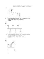
2-37
Year

0.00
1.00
2.00
3.00

Capital Costs
-20
0
0
0

O&M
0
-2.5
-2.5
-2.5

Overhaul
0
0
0
0

Total
-$5,000
-$7,000
-$8,000
-$8,000
+$5,000

4.00
5.00
6.00
7.00

0
0
0
2

-2.5
-2.5
-2.5
-2.5

-5
0
0
0

Cash Flow ($1,000)

10
5
0

Overhaul

-5

O&M
Capital Costs

-10
-15
-20
00 .00 .00 .00 .00 .00 .00 .00
0.
1
2
3
4
5
6
7

Year

2-38
Year
0
1
2
3
4
5
6
7
8

9
10

CapitalCosts
-225

100

O&M
-85
-85
-85
-85
-85
-85
-85
-85
-85
-85

Overhaul

-75

Benefits
190
190
190
190
190

190
190
190
190
190


400

300

200

Benefits

100

Overhaul
O&M
0

Capital Costs
0

1

2

3

4

5

6

7

8

9

10

-100

-200

-300

2-39
Each student’s answers will be different depending on their university and life situation.
As an example:
First Costs: tuition costs, fees, books, supplies, board (if paid ahead)
O & M Costs: monthly living expenses, rent (if applicable)
Salvage Value: selling books back to student union, etc.
Revenues: wages & tips, etc.
Overhauls: periodic (random or planned) mid-term expenses
The cash flow diagram is left to the student.