Solution manual fundamentals of physics extended, 8th editionch02

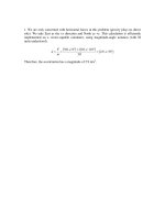
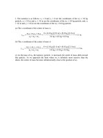
1. The speed (assumed constant) is (90 km/h)(1000 m/km) ⁄ (3600 s/h) = 25 m/s. Thus,
during 0.50 s, the car travels (0.50)(25) ≈ 13 m.


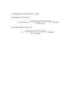
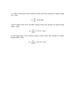
2. Huber’s speed is
v0=(200 m)/(6.509 s)=30.72 m/s = 110.6 km/h,
where we have used the conversion factor 1 m/s = 3.6 km/h. Since Whittingham beat
Huber by 19.0 km/h, his speed is v1=(110.6 + 19.0)=129.6 km/h, or 36 m/s (1 km/h =
0.2778 m/s). Thus, the time through a distance of 200 m for Whittingham is
∆t =

∆ x 200 m
=
= 5.554 s.
v1 36 m/s


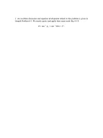
3. We use Eq. 2-2 and Eq. 2-3. During a time tc when the velocity remains a positive
constant, speed is equivalent to velocity, and distance is equivalent to displacement,
with ∆x = v tc.
(a) During the first part of the motion, the displacement is ∆x1 = 40 km and the time
interval is

t1 =

(40 km)
= 133
. h.
(30 km / h)

During the second part the displacement is ∆x2 = 40 km and the time interval is

t2 =

(40 km)
= 0.67 h.
(60 km / h)

Both displacements are in the same direction, so the total displacement is
∆x = ∆x1 + ∆x2 = 40 km + 40 km = 80 km.
The total time for the trip is t = t1 + t2 = 2.00 h. Consequently, the average velocity is
vavg =

(80 km)
= 40 km / h.
(2.0 h)

(b) In this example, the numerical result for the average speed is the same as the
average velocity 40 km/h.
(c) As shown below, the graph consists of two contiguous line segments, the first
having a slope of 30 km/h and connecting the origin to (t1, x1) = (1.33 h, 40 km) and
the second having a slope of 60 km/h and connecting (t1, x1) to (t, x) = (2.00 h, 80 km).
From the graphical point of view , the slope of the dashed line drawn from the origin
to (t, x) represents the average velocity.


4. Average speed, as opposed to average velocity, relates to the total distance, as
opposed to the net displacement. The distance D up the hill is, of course, the same as
the distance down the hill, and since the speed is constant (during each stage of the
motion) we have speed = D/t. Thus, the average speed is
Dup + Ddown
t up + t down

=

2D
D
D
+
vup vdown

which, after canceling D and plugging in vup = 40 km/h and vdown = 60 km/h, yields 48
km/h for the average speed.


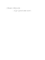
5. Using x = 3t – 4t2 + t3 with SI units understood is efficient (and is the approach we
will use), but if we wished to make the units explicit we would write x = (3 m/s)t – (4
m/s2)t2 + (1 m/s3)t3.We will quote our answers to one or two significant figures, and
not try to follow the significant figure rules rigorously.
(a) Plugging in t = 1 s yields x = 3 – 4 + 1 = 0.
(b) With t = 2 s we get x = 3(2) – 4(2)2+(2)3 = –2 m.
(c) With t = 3 s we have x = 0 m.
(d) Plugging in t = 4 s gives x = 12 m.
For later reference, we also note that the position at t = 0 is x = 0.
(e) The position at t = 0 is subtracted from the position at t = 4 s to find the
displacement ∆x = 12 m.
(f) The position at t = 2 s is subtracted from the position at t = 4 s to give the
displacement ∆x = 14 m. Eq. 2-2, then, leads to
vavg =

∆x 14
=

= 7 m / s.
∆t
2

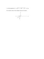
(g) The horizontal axis is 0 ≤ t ≤ 4 with SI units understood.
Not shown is a straight line drawn from the point at (t, x) = (2, –2) to the highest point
shown (at t = 4 s) which would represent the answer for part (f).


6. (a) Using the fact that time = distance/velocity while the velocity is constant, we
find
vavg =

73.2 m + 73.2 m
= 1.74 m/s.
73.2 m
73.2 m
1.22 m/s + 3.05 m

(b) Using the fact that distance = vt while the velocity v is constant, we find
vavg =

(122
. m / s)(60 s) + (3.05 m / s)(60 s)
= 2.14 m / s.
120 s

(c) The graphs are shown below (with meters and seconds understood). The first
consists of two (solid) line segments, the first having a slope of 1.22 and the second
having a slope of 3.05. The slope of the dashed line represents the average velocity (in

both graphs). The second graph also consists of two (solid) line segments, having the
same slopes as before — the main difference (compared to the first graph) being that
the stage involving higher-speed motion lasts much longer.


7. We use the functional notation x(t), v(t) and a(t) in this solution, where the latter
two quantities are obtained by differentiation:

bg

vt =

bg

bg

dx t
dv t
= − 12t and a t =
= − 12
dt
dt

bg

with SI units understood.
(a) From v(t) = 0 we find it is (momentarily) at rest at t = 0.
(b) We obtain x(0) = 4.0 m
(c) and (d) Requiring x(t) = 0 in the expression x(t) = 4.0 – 6.0t2 leads to t = ±0.82 s
for the times when the particle can be found passing through the origin.

(e) We show both the asked-for graph (on the left) as well as the “shifted” graph
which is relevant to part (f). In both cases, the time axis is given by –3 ≤ t ≤ 3 (SI
units understood).

(f) We arrived at the graph on the right (shown above) by adding 20t to the x(t)
expression.
(g) Examining where the slopes of the graphs become zero, it is clear that the shift
causes the v = 0 point to correspond to a larger value of x (the top of the second curve
shown in part (e) is higher than that of the first).


8. The values used in the problem statement make it easy to see that the first part of
the trip (at 100 km/h) takes 1 hour, and the second part (at 40 km/h) also takes 1 hour.
Expressed in decimal form, the time left is 1.25 hour, and the distance that remains is
160 km. Thus, a speed of 160/1.25 = 128 km/h is needed.


9. Converting to seconds, the running times are t1 = 147.95 s and t2 = 148.15 s,
respectively. If the runners were equally fast, then
savg1 = savg 2

Ÿ

L1 L2
= .
t1 t2

From this we obtain

§t

·
§ 148.15 ·
L2 − L1 = ¨ 2 − 1 ¸ L1 = ¨
− 1 ¸ L1 = 0.00135 L1 ≈ 1.4 m
© 147.95 ¹
© t1
¹
where we set L1 ≈ 1000 m in the last step. Thus, if L1 and L2 are no different than
about 1.4 m, then runner 1 is indeed faster than runner 2. However, if L1 is shorter
than L2 by more than 1.4 m, then runner 2 would actually be faster.


10. Recognizing that the gap between the trains is closing at a constant rate of 60
km/h, the total time which elapses before they crash is t = (60 km)/(60 km/h) = 1.0 h.
During this time, the bird travels a distance of x = vt = (60 km/h)(1.0 h) = 60 km.


11. (a) Denoting the travel time and distance from San Antonio to Houston as T and D,
respectively, the average speed is
savg1 =

D (55 km / h) T2 + ( 90 km / h) T2
=
= 72.5 km / h
T
T

which should be rounded to 73 km/h.
(b) Using the fact that time = distance/speed while the speed is constant, we find
savg 2 =

D
=
T

D/2
55 km/h

D
= 68.3 km/h
/2
+ 90Dkm/h

which should be rounded to 68 km/h.
(c) The total distance traveled (2D) must not be confused with the net displacement
(zero). We obtain for the two-way trip
savg =

2D
= 70 km/h.
+ 68.3Dkm/h

D
72.5 km/h

(d) Since the net displacement vanishes, the average velocity for the trip in its entirety
is zero.
(e) In asking for a sketch, the problem is allowing the student to arbitrarily set the
distance D (the intent is not to make the student go to an Atlas to look it up); the
student can just as easily arbitrarily set T instead of D, as will be clear in the following

discussion. In the interest of saving space, we briefly describe the graph (with
kilometers-per-hour understood for the slopes): two contiguous line segments, the
first having a slope of 55 and connecting the origin to (t1, x1) = (T/2, 55T/2) and the
second having a slope of 90 and connecting (t1, x1) to (T, D) where D = (55 + 90)T/2.
The average velocity, from the graphical point of view, is the slope of a line drawn
from the origin to (T, D). The graph (not drawn to scale) is depicted below:


12. We use Eq. 2-4. to solve the problem.
(a) The velocity of the particle is
v=

dx d
=
(4 − 12t + 3t 2 ) = −12 + 6t .
dt dt

Thus, at t = 1 s, the velocity is v = (–12 + (6)(1)) = –6 m/s.
(b) Since v < 0, it is moving in the negative x direction at t = 1 s.
(c) At t = 1 s, the speed is |v| = 6 m/s.
(d) For 0 < t < 2 s, |v| decreases until it vanishes. For 2 < t < 3 s, |v| increases from
zero to the value it had in part (c). Then, |v| is larger than that value for t > 3 s.
(e) Yes, since v smoothly changes from negative values (consider the t = 1 result) to
positive (note that as t → + ∞, we have v → + ∞). One can check that v = 0 when
t = 2 s.
(f) No. In fact, from v = –12 + 6t, we know that v > 0 for t > 2 s.


13. We use Eq. 2-2 for average velocity and Eq. 2-4 for instantaneous velocity, and
work with distances in centimeters and times in seconds.

(a) We plug into the given equation for x for t = 2.00 s and t = 3.00 s and obtain x2 =
21.75 cm and x3 = 50.25 cm, respectively. The average velocity during the time
interval 2.00 ≤ t ≤ 3.00 s is
vavg =

∆x 50.25 cm − 2175
. cm
=
∆t
3.00 s − 2.00 s

which yields vavg = 28.5 cm/s.
(b) The instantaneous velocity is v =
(4.5)(2.00)2 = 18.0 cm/s.

dx
dt

= 4.5t 2 , which, at time t = 2.00 s, yields v =

(c) At t = 3.00 s, the instantaneous velocity is v = (4.5)(3.00)2 = 40.5 cm/s.
(d) At t = 2.50 s, the instantaneous velocity is v = (4.5)(2.50)2 = 28.1 cm/s.
(e) Let tm stand for the moment when the particle is midway between x2 and x3 (that is,
when the particle is at xm = (x2 + x3)/2 = 36 cm). Therefore,
. t m3
xm = 9.75 + 15

Ÿ

t m = 2.596

in seconds. Thus, the instantaneous speed at this time is v = 4.5(2.596)2 = 30.3 cm/s.
(f) The answer to part (a) is given by the slope of the straight line between t = 2 and t
= 3 in this x-vs-t plot. The answers to parts (b), (c), (d) and (e) correspond to the
slopes of tangent lines (not shown but easily imagined) to the curve at the appropriate
points.


14. We use the functional notation x(t), v(t) and a(t) and find the latter two quantities
by differentiating:

bg

vt =

b g = − 15t

dx t
t

2

+ 20

and

bg

at =

b g = − 30t

dv t
dt

with SI units understood. These expressions are used in the parts that follow.
(a) From 0 = − 15t 2 + 20 , we see that the only positive value of t for which the
. s.
particle is (momentarily) stopped is t = 20 / 15 = 12
(b) From 0 = – 30t, we find a(0) = 0 (that is, it vanishes at t = 0).
(c) It is clear that a(t) = – 30t is negative for t > 0
(d) The acceleration a(t) = – 30t is positive for t < 0.
(e) The graphs are shown below. SI units are understood.


15. We represent its initial direction of motion as the +x direction, so that v0 = +18 m/s
and v = –30 m/s (when t = 2.4 s). Using Eq. 2-7 (or Eq. 2-11, suitably interpreted) we
find
aavg =

( −30) − ( +18)
= − 20 m / s2
2.4

which indicates that the average acceleration has magnitude 20 m/s2 and is in the
opposite direction to the particle’s initial velocity.


d
dx

16. Using the general property
v=

FG
H

exp(bx ) = b exp(bx ) , we write

IJ
K

FG IJ
H K

dx
d (19t )
de − t
=
⋅ e − t + (19t ) ⋅
dt
dt
dt

.

If a concern develops about the appearance of an argument of the exponential (–t)
apparently having units, then an explicit factor of 1/T where T = 1 second can be
inserted and carried through the computation (which does not change our answer).
The result of this differentiation is

v = 16(1 − t )e − t
with t and v in SI units (s and m/s, respectively). We see that this function is zero
when t = 1 s. Now that we know when it stops, we find out where it stops by
plugging our result t = 1 into the given function x = 16te–t with x in meters. Therefore,
we find x = 5.9 m.


17. (a) Taking derivatives of x(t) = 12t2 – 2t3 we obtain the velocity and the
acceleration functions:
v(t) = 24t – 6t2

and

a(t) = 24 – 12t

with length in meters and time in seconds. Plugging in the value t = 3 yields
x(3) = 54 m .
(b) Similarly, plugging in the value t = 3 yields v(3) = 18 m/s.
(c) For t = 3, a(3) = –12 m/s2.
(d) At the maximum x, we must have v = 0; eliminating the t = 0 root, the velocity
equation reveals t = 24/6 = 4 s for the time of maximum x. Plugging t = 4 into the
equation for x leads to x = 64 m for the largest x value reached by the particle.
(e) From (d), we see that the x reaches its maximum at t = 4.0 s.
(f) A maximum v requires a = 0, which occurs when t = 24/12 = 2.0 s. This, inserted
into the velocity equation, gives vmax = 24 m/s.
(g) From (f), we see that the maximum of v occurs at t = 24/12 = 2.0 s.
(h) In part (e), the particle was (momentarily) motionless at t = 4 s. The acceleration at
that time is readily found to be 24 – 12(4) = –24 m/s2.
(i) The average velocity is defined by Eq. 2-2, so we see that the values of x at t = 0
and t = 3 s are needed; these are, respectively, x = 0 and x = 54 m (found in part (a)).

Thus,
vavg =

54 − 0
= 18 m/s .
3−0


18. We use Eq. 2-2 (average velocity) and Eq. 2-7 (average acceleration). Regarding
our coordinate choices, the initial position of the man is taken as the origin and his
direction of motion during 5 min ≤ t ≤ 10 min is taken to be the positive x direction.
We also use the fact that ∆x = v∆t ' when the velocity is constant during a time
interval ∆t' .
(a) The entire interval considered is ∆t = 8 – 2 = 6 min which is equivalent to 360 s,
whereas the sub-interval in which he is moving is only ∆t' = 8 − 5 = 3min = 180 s.
His position at t = 2 min is x = 0 and his position at t = 8 min is x = v∆t' =
(2.2)(180) = 396 m . Therefore,

vavg =

396 m − 0
= 110
. m / s.
360 s

(b) The man is at rest at t = 2 min and has velocity v = +2.2 m/s at t = 8 min. Thus,
keeping the answer to 3 significant figures,
aavg =

2.2 m / s − 0

= 0.00611 m / s2 .
360 s

(c) Now, the entire interval considered is ∆t = 9 – 3 = 6 min (360 s again), whereas the
sub-interval in which he is moving is ∆t' = 9 − 5 = 4 min = 240 s). His position at
t = 3 min is x = 0 and his position at t = 9 min is x = v∆t ' = (2.2)(240) = 528 m .
Therefore,
vavg =

528 m − 0
= 147
. m / s.
360 s

(d) The man is at rest at t = 3 min and has velocity v = +2.2 m/s at t = 9 min.
Consequently, aavg = 2.2/360 = 0.00611 m/s2 just as in part (b).
(e) The horizontal line near the bottom of this x-vs-t graph represents the man
standing at x = 0 for 0 ≤ t < 300 s and the linearly rising line for 300 ≤ t ≤ 600 s
represents his constant-velocity motion. The dotted lines represent the answers to part
(a) and (c) in the sense that their slopes yield those results.


The graph of v-vs-t is not shown here, but would consist of two horizontal “steps”
(one at v = 0 for 0 ≤ t < 300 s and the next at v = 2.2 m/s for 300 ≤ t ≤ 600 s). The
indications of the average accelerations found in parts (b) and (d) would be dotted
lines connecting the “steps” at the appropriate t values (the slopes of the dotted lines
representing the values of aavg).


19. In this solution, we make use of the notation x(t) for the value of x at a particular t.

The notations v(t) and a(t) have similar meanings.
(a) Since the unit of ct2 is that of length, the unit of c must be that of length/time2, or
m/s2 in the SI system.
(b) Since bt3 has a unit of length, b must have a unit of length/time3, or m/s3.
(c) When the particle reaches its maximum (or its minimum) coordinate its velocity is
zero. Since the velocity is given by v = dx/dt = 2ct – 3bt2, v = 0 occurs for t = 0 and
for

t=

2c 2(3.0 m / s2 )
. s.
=
= 10
3b 3(2.0 m / s3 )

For t = 0, x = x0 = 0 and for t = 1.0 s, x = 1.0 m > x0. Since we seek the maximum, we
reject the first root (t = 0) and accept the second (t = 1s).
(d) In the first 4 s the particle moves from the origin to x = 1.0 m, turns around, and
goes back to
x(4 s) = (3.0 m / s 2 )(4.0 s) 2 − (2.0 m / s 3 )(4.0 s) 3 = − 80 m .
The total path length it travels is 1.0 m + 1.0 m + 80 m = 82 m.
(e) Its displacement is ∆x = x2 – x1, where x1 = 0 and x2 = –80 m. Thus, ∆x = −80 m .
The velocity is given by v = 2ct – 3bt2 = (6.0 m/s2)t – (6.0 m/s3)t2.
(f) Plugging in t = 1 s, we obtain
v(1 s) = (6.0 m/s 2 )(1.0 s) − (6.0 m/s 3 )(1.0 s) 2 = 0.
(g) Similarly, v(2 s) = (6.0 m/s 2 )(2.0 s) − (6.0 m/s3 )(2.0 s) 2 = − 12m/s .
(h) v(3 s) = (6.0 m/s 2 )(3.0 s) − (6.0 m/s 3 )(3.0 s) 2 = − 36.0 m/s .
(i) v(4 s) = (6.0 m/s 2 )(4.0 s) − (6.0 m/s3 )(4.0 s) 2 = −72 m/s .
The acceleration is given by a = dv/dt = 2c – 6b = 6.0 m/s2 – (12.0 m/s3)t.

(j) Plugging in t = 1 s, we obtain
a (1 s) = 6.0 m/s 2 − (12.0 m/s3 )(1.0 s) = − 6.0 m/s 2 .


(k) a (2 s) = 6.0 m/s 2 − (12.0 m/s3 )(2.0 s) = − 18 m/s 2 .
(l) a (3 s) = 6.0 m/s 2 − (12.0 m/s3 )(3.0 s) = −30 m/s 2 .
(m) a (4 s) = 6.0 m/s 2 − (12.0 m/s3 )(4.0 s) = − 42 m/s 2 .


20. The constant-acceleration condition permits the use of Table 2-1.
(a) Setting v = 0 and x0 = 0 in v 2 = v02 + 2a ( x − x0 ) , we find
x=−

FG
H

IJ
K

1 v 02
1 5.00 × 10 6
.
m.
=−
= 0100
2 a
2 −125
. × 1014

Since the muon is slowing, the initial velocity and the acceleration must have opposite

signs.
(b) Below are the time-plots of the position x and velocity v of the muon from the
moment it enters the field to the time it stops. The computation in part (a) made no
reference to t, so that other equations from Table 2-1 (such as v = v0 + at and
x = v0 t + 12 at 2 ) are used in making these plots.


21. We use v = v0 + at, with t = 0 as the instant when the velocity equals +9.6 m/s.
(a) Since we wish to calculate the velocity for a time before t = 0, we set t = –2.5 s.
Thus, Eq. 2-11 gives

c

h

c

h

v = (9.6 m / s) + 3.2 m / s2 ( −2.5 s) = 16
. m / s.

(b) Now, t = +2.5 s and we find
v = (9.6 m / s) + 3.2 m / s2 (2.5 s) = 18 m / s.


22. We take +x in the direction of motion, so v0 = +24.6 m/s and a = – 4.92 m/s2. We
also take x0 = 0.
(a) The time to come to a halt is found using Eq. 2-11:
0 = v0 + at Ÿ t =

24.6
= 5.00 s .
− 4.92

(b) Although several of the equations in Table 2-1 will yield the result, we choose Eq.
2-16 (since it does not depend on our answer to part (a)).
0 = v02 + 2ax Ÿ x = −

24.62
= 61.5 m .
2 ( − 4.92 )

(c) Using these results, we plot v0t + 12 at 2 (the x graph, shown next, on the left) and
v0 + at (the v graph, on the right) over 0 ≤ t ≤ 5 s, with SI units understood.


23. The constant acceleration stated in the problem permits the use of the equations in
Table 2-1.
(a) We solve v = v0 + at for the time:
t=

v − v0
=
a

1
10

(3.0 × 10 8 m / s)

. × 10 6 s
= 31
2
9.8 m / s

which is equivalent to 1.2 months.
(b) We evaluate x = x0 + v0 t + 12 at 2 , with x0 = 0. The result is
x=

1
( 9.8 m/s2 ) (3.1×106 s)2 = 4.6 ×1013 m .
2