Solution manual fundamentals of physics extended, 8th editionch10

1. (a) The second hand of the smoothly running watch turns through 2π radians during
60 s . Thus,

ω=

2π
= 0.105 rad/s.
60

(b) The minute hand of the smoothly running watch turns through 2π radians during
3600 s . Thus,

ω=

2π
= 1.75 × 10 −3 rad / s.
3600

(c) The hour hand of the smoothly running 12-hour watch turns through 2π radians
during 43200 s. Thus,

ω=

2π
= 145
. × 10 −4 rad / s.
43200


2. The problem asks us to assume vcom and ω are constant. For consistency of units, we
write

b

vcom = 85 mi h

ft mi I
g FGH 5280
J = 7480 ft min .
60 min h K

Thus, with ∆x = 60 ft , the time of flight is t = ∆x vcom = 60 7480 = 0.00802 min . During
that time, the angular displacement of a point on the ball’s surface is

b

gb

g

θ = ωt = 1800 rev min 0.00802 min ≈ 14 rev .


3. We have ω = 10π rad/s. Since α = 0, Eq. 10-13 gives
∆θ = ωt = (10π rad/s)(n ∆t), for n = 1, 2, 3, 4, 5, ….
For ∆t = 0.20 s, we always get an integer multiple of 2π (and 2π radians corresponds to 1
revolution).
(a) At f1 ∆θ = 2π rad the dot appears at the “12:00” (straight up) position.
(b) At f2, ∆θ = 4π rad and the dot appears at the “12:00” position.
∆t = 0.050 s, and we explicitly include the 1/2π conversion (to revolutions) in this
calculation:

1
∆θ = ωt = (10π rad/s)n(0.050 s)§©2π·¹ = ¼ , ½ , ¾ , 1, … (revs)

(c) At f1(n=1), ∆θ = 1/4 rev and the dot appears at the “3:00” position.
(d) At f2(n=2), ∆θ = 1/2 rev and the dot appears at the “6:00” position.
(e) At f3(n=3), ∆θ = 3/4 rev and the dot appears at the “9:00” position.
(f) At f4(n=4), ∆θ = 1 rev and the dot appears at the “12:00” position.
Now ∆t = 0.040 s, and we have
1
∆θ = ωt = (10π rad/s)n(0.040 s)§©2π·¹ = 0.2 , 0.4 , 0.6 , 0.8, 1, … (revs)

Note that 20% of 12 hours is 2.4 h = 2 h and 24 min.
(g) At f1(n=1), ∆θ = 0.2 rev and the dot appears at the “2:24” position.
(h) At f2(n=2), ∆θ = 0.4 rev and the dot appears at the “4:48” position.
(i) At f3(n=3), ∆θ = 0.6 rev and the dot appears at the “7:12” position.
(j) At f4(n=4), ∆θ = 0.8 rev and the dot appears at the “9:36” position.
(k) At f5(n=5), ∆θ = 1.0 rev and the dot appears at the “12:00” position.


4. If we make the units explicit, the function is

b

g c

h c

h

θ = 4.0 rad / s t − 3.0 rad / s2 t 2 + 10

. rad / s3 t 3
but generally we will proceed as shown in the problem—letting these units be understood.
Also, in our manipulations we will generally not display the coefficients with their proper
number of significant figures.
(a) Eq. 10-6 leads to

ω=

d
4t − 3t 2 + t 3 = 4 − 6t + 3t 2 .
dt

c

h

Evaluating this at t = 2 s yields ω2 = 4.0 rad/s.
(b) Evaluating the expression in part (a) at t = 4 s gives ω4 = 28 rad/s.
(c) Consequently, Eq. 10-7 gives

α avg =

ω4 −ω2
4−2

= 12 rad / s2 .

(d) And Eq. 10-8 gives

α=

dω d
=
4 − 6t + 3t 2 = −6 + 6t .
dt dt

c

h

Evaluating this at t = 2 s produces α2 = 6.0 rad/s2.
(e) Evaluating the expression in part (d) at t = 4 s yields α4 = 18 rad/s2. We note that our
answer for αavg does turn out to be the arithmetic average of α2 and α4 but point out that
this will not always be the case.


5. Applying Eq. 2-15 to the vertical axis (with +y downward) we obtain the free-fall time:

∆y = v0 y t +

1 2
2(10)
gt Ÿ t =
= 14
. s.
2
9.8

Thus, by Eq. 10-5, the magnitude of the average angular velocity is

ω avg =

( 2.5) ( 2π )
= 11 rad / s.
14
.


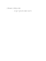
6. If we make the units explicit, the function is

θ = 2.0 rad + ( 4.0 rad/s 2 ) t 2 + ( 2.0 rad/s3 ) t 3
but in some places we will proceed as indicated in the problem—by letting these units be
understood.
(a) We evaluate the function θ at t = 0 to obtain θ0 = 2.0 rad.
(b) The angular velocity as a function of time is given by Eq. 10-6:

ω=

dθ
= ( 8.0 rad/s 2 ) t + ( 6.0 rad/s3 ) t 2
dt

which we evaluate at t = 0 to obtain ω0 = 0.
(c) For t = 4.0 s, the function found in the previous part is ω4 = (8.0)(4.0) + (6.0)(4.0)2 =
128 rad/s. If we round this to two figures, we obtain ω4 ≈ 1.3 × 102 rad/s.
(d) The angular acceleration as a function of time is given by Eq. 10-8:

α=

dω

= 8.0 rad/s 2 + (12 rad/s3 ) t
dt

which yields α2 = 8.0 + (12)(2.0) = 32 rad/s2 at t = 2.0 s.
(e) The angular acceleration, given by the function obtained in the previous part, depends
on time; it is not constant.


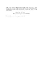
7. (a) To avoid touching the spokes, the arrow must go through the wheel in not more
than
∆t =

1 / 8 rev
= 0.050 s.
2.5 rev / s

The minimum speed of the arrow is then vmin =

20 cm
= 400 cm / s = 4.0 m / s.
0.050 s

(b) No—there is no dependence on radial position in the above computation.


8. (a) With ω = 0 and α = – 4.2 rad/s2, Eq. 10-12 yields t = –ωo/α = 3.00 s.
(b) Eq. 10-4 gives θ − θo = − ωo2 / 2α = 18.9 rad.


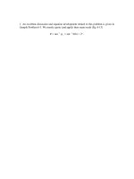
9. (a) We assume the sense of rotation is positive. Applying Eq. 10-12, we obtain

ω = ω0 + α t Ÿ α =

3000 − 1200
= 9.0 ×103 rev/min 2 .
12 / 60

(b) And Eq. 10-15 gives
1
2

1
2

θ = (ω 0 + ω ) t = (1200 + 3000)

FG 12 IJ = 4.2 ×10
H 60K

2

rev.


10. We assume the sense of initial rotation is positive. Then, with ω0 = +120 rad/s and ω
= 0 (since it stops at time t), our angular acceleration (‘‘deceleration’’) will be negativevalued: α = – 4.0 rad/s2.
(a) We apply Eq. 10-12 to obtain t.

ω = ω0 + α t

Ÿ t=

0 − 120
= 30 s.
−4.0

(b) And Eq. 10-15 gives
1
1
θ = (ω 0 + ω ) t = (120 + 0) (30) = 1.8 × 103 rad.
2
2

Alternatively, Eq. 10-14 could be used if it is desired to only use the given information
(as opposed to using the result from part (a)) in obtaining θ. If using the result of part (a)
is acceptable, then any angular equation in Table 10-1 (except Eq. 10-12) can be used to
find θ.


11. We assume the sense of rotation is positive, which (since it starts from rest) means all
quantities (angular displacements, accelerations, etc.) are positive-valued.
(a) The angular acceleration satisfies Eq. 10-13:
1
25 rad = α (5.0 s) 2 Ÿ α = 2.0 rad/s 2 .
2

(b) The average angular velocity is given by Eq. 10-5:

ω avg =

∆θ 25 rad
=
= 5.0 rad / s.
∆t
5.0 s

(c) Using Eq. 10-12, the instantaneous angular velocity at t = 5.0 s is

c

h

ω = 2.0 rad / s2 (5.0 s) = 10 rad / s .
(d) According to Eq. 10-13, the angular displacement at t = 10 s is
1
1
θ = ω 0 + αt 2 = 0 + (2.0) (10) 2 = 100 rad.
2
2

Thus, the displacement between t = 5 s and t = 10 s is ∆θ = 100 – 25 = 75 rad.


12. (a) Eq. 10-13 gives

θ − θo = ωo t +

1 2
αt
2

1

= 0 + 2 (1.5 rad/s²) t12

where θ − θo = (2 rev)(2π rad/rev). Therefore, t1 = 4.09 s.
(b) We can find the time to go through a full 4 rev (using the same equation to solve for a
new time t2) and then subtract the result of part (a) for t1 in order to find this answer.
1

(4 rev)(2π rad/rev) = 0 + 2 (1.5 rad/s²) t22
Thus, the answer is 5.789 – 4.093 ≈ 1.70 s.

Ÿ

t2 = 5.789 s.


13. We take t = 0 at the start of the interval and take the sense of rotation as positive.
Then at the end of the t = 4.0 s interval, the angular displacement is θ = ω 0 t + 21 αt 2 . We
solve for the angular velocity at the start of the interval:

ω0 =

θ − 12 α t 2
t

=

(

120 rad − 12 3.0 rad/s 2

) ( 4.0 s )

4.0 s

2

= 24 rad/s.

We now use ω = ω0 + α t (Eq. 10-12) to find the time when the wheel is at rest:
t=−

ω0
24 rad / s
=−
= −8.0 s.
3.0 rad / s2
α

That is, the wheel started from rest 8.0 s before the start of the described 4.0 s interval.


14. (a) The upper limit for centripetal acceleration (same as the radial acceleration – see
Eq. 10-23) places an upper limit of the rate of spin (the angular velocity ω) by
considering a point at the rim (r = 0.25 m). Thus, ωmax = a/r = 40 rad/s. Now we apply
Eq. 10-15 to first half of the motion (where ωo = 0):

θ − θo =

1
(ωo
2

+ ω)t Ÿ 400 rad =

1
(0
2

+ 40 rad/s)t

which leads to t = 20 s. The second half of the motion takes the same amount of time
(the process is essentially the reverse of the first); the total time is therefore 40 s.
(b) Considering the first half of the motion again, Eq. 10-11 leads to

ω = ωo + α t Ÿ α =

40 rad/s
= 2.0 rad/s2 .
20 s


15. The wheel has angular velocity ω0 = +1.5 rad/s = +0.239 rev/s2 at t = 0, and has
constant value of angular acceleration α < 0, which indicates our choice for positive
sense of rotation. At t1 its angular displacement (relative to its orientation at t = 0) is θ1 =
+20 rev, and at t2 its angular displacement is θ2 = +40 rev and its angular velocity is
ω2 = 0 .
(a) We obtain t2 using Eq. 10-15:

θ2 =

1
2(40)
ω 0 + ω 2 t2 Ÿ t2 =
2
0.239

b

g

which yields t2 = 335 s which we round off to t2 ≈ 3.4 ×10 2 s .
(b) Any equation in Table 10-1 involving α can be used to find the angular acceleration;
we select Eq. 10-16.
1
2(40)
θ 2 = ω 2t2 − α t22 Ÿ α = −
2
3352

which yields α = –7.12 × 10–4 rev/s2 which we convert to α = – 4.5 × 10–3 rad/s2.
(c) Using θ 1 = ω 0t1 + 21 αt12 (Eq. 10-13) and the quadratic formula, we have

t1 =

−ω 0 ± ω 20 + 2θ 1α

α

=

b gc

−0.239 ± 0.239 2 + 2 20 −7.12 × 10 −4
−7.12 × 10

h

−4

which yields two positive roots: 98 s and 572 s. Since the question makes sense only if t1
< t2 we conclude the correct result is t1 = 98 s.


16. The wheel starts turning from rest (ω0 = 0) at t = 0, and accelerates uniformly at α > 0,
which makes our choice for positive sense of rotation. At t1 its angular velocity is ω1 =
+10 rev/s, and at t2 its angular velocity is ω2 = +15 rev/s. Between t1 and t2 it turns
through ∆θ = 60 rev, where t2 – t1 = ∆t.
(a) We find α using Eq. 10-14:

ω22 = ω12 + 2α∆θ Ÿ α =

152 − 102
2(60)

which yields α = 1.04 rev/s2 which we round off to 1.0 rev/s2.
(b) We find ∆t using Eq. 10-15:
∆θ =

1
2(60)
ω 1 + ω 2 ∆t Ÿ ∆ t =
= 4.8 s.
2
10 + 15

b

g

(c) We obtain t1 using Eq. 10-12: ω1 = ω 0 + α t1 Ÿ t1 =

10
= 9.6 s.
1.04

(d) Any equation in Table 10-1 involving θ can be used to find θ1 (the angular
displacement during 0 ≤ t ≤ t1); we select Eq. 10-14.

ω12 = ω 02 + 2αθ1 Ÿ θ1 =

102
= 48 rev.
2(1.04)


17. The problem has (implicitly) specified the positive sense of rotation. The angular
acceleration of magnitude 0.25 rad/s2 in the negative direction is assumed to be constant

over a large time interval, including negative values (for t).
(a) We specify θmax with the condition ω = 0 (this is when the wheel reverses from
positive rotation to rotation in the negative direction). We obtain θmax using Eq. 10-14:

θ max = −

4.7 2
ω 2o
=−
= 44 rad.
2α
2( −0.25)

(b) We find values for t1 when the angular displacement (relative to its orientation at t = 0)
is θ1 = 22 rad (or 22.09 rad if we wish to keep track of accurate values in all intermediate
steps and only round off on the final answers). Using Eq. 10-13 and the quadratic formula,
we have
−ω o ± ω o2 + 2θ1α
1 2
θ1 = ω ot1 + α t1 Ÿ t1 =
α
2
which yields the two roots 5.5 s and 32 s. Thus, the first time the reference line will be at
θ1 = 22 rad is t = 5.5 s.
(c) The second time the reference line will be at θ1 = 22 rad is t = 32 s.
(d) We find values for t2 when the angular displacement (relative to its orientation at t = 0)
is θ2 = –10.5 rad. Using Eq. 10-13 and the quadratic formula, we have
1
2

θ 2 = ωot2 + α t22 Ÿ t2 =

−ω o ± ω o2 + 2θ 2α

α

which yields the two roots –2.1 s and 40 s. Thus, at t = –2.1 s the reference line will be at
θ2 = –10.5 rad.
(e) At t = 40 s the reference line will be at θ2 = –10.5 rad.
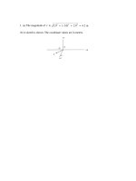
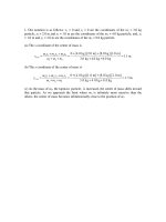
(f) With radians and seconds understood, the graph of θ versus t is shown below (with the
points found in the previous parts indicated as small circles).



18. The wheel starts turning from rest (ω0 = 0) at t = 0, and accelerates uniformly at
α = 2.00 rad/s 2 .Between t1 and t2 the wheel turns through ∆θ = 90.0 rad, where t2 – t1 =
∆t = 3.00 s.
(a) We use Eq. 10-13 (with a slight change in notation) to describe the motion for t1 ≤ t ≤
t2:
∆θ α∆t
1
∆ θ = ω 1 ∆t + α ( ∆t ) 2 Ÿ ω 1 =
−
∆t
2
2

which we plug into Eq. 10-12, set up to describe the motion during 0 ≤ t ≤ t1:

ω1 = ω0 + α t1 Ÿ

∆θ α ∆t
−
= α t1 Ÿ
∆t
2

90.0 (2.00) (3.00)
−
= (2.00) t1
3.00
2

yielding t1 = 13.5 s.
(b) Plugging into our expression for ω1 (in previous part) we obtain

ω1 =

∆θ α∆t 90.0 (2.00)(3.00)
−
=
−
= 27.0 rad / s.
∆t
2
3.00
2


19. We assume the given rate of 1.2 × 10–3 m/y is the linear speed of the top; it is also

possible to interpret it as just the horizontal component of the linear speed but the
difference between these interpretations is arguably negligible. Thus, Eq. 10-18 leads to
12
. × 10−3 m / y
ω=
= 2.18 × 10−5 rad / y
55 m
which we convert (since there are about 3.16 × 107 s in a year) to ω = 6.9 × 10–13 rad/s.


1

20. Converting 333 rev/min to radians-per-second, we get ω = 3.49 rad/s. Combining

v = ω r (Eq. 10-18) with ∆t = d/v where ∆t is the time between bumps (a distance d apart),
we arrive at the rate of striking bumps:
1
ωr
= d
∆t

≈ 199 /s.


21. (a) We obtain

ω=

(200 rev / min)(2 π rad / rev)
= 20.9 rad / s.

60 s / min

(b) With r = 1.20/2 = 0.60 m, Eq. 10-18 leads to v = rω = (0.60)(20.9) = 12.5 m/s.
(c) With t = 1 min, ω = 1000 rev/min and ω0 = 200 rev/min, Eq. 10-12 gives

α=

ω −ωo
= 800 rev / min 2 .
t

(d) With the same values used in part (c), Eq. 10-15 becomes

θ=

1
1
ω o + ω t = (200 + 100)(1) = 600 rev.
2
2

b

g


22. (a) Using Eq. 10-6, the angular velocity at t = 5.0s is

ω=

dθ
dt

=
t =5.0

d
0.30t 2
dt

c

h

= 2(0.30)(5.0) = 3.0 rad / s.
t =5.0

(b) Eq. 10-18 gives the linear speed at t = 5.0s: v = ω r = (3.0 rad/s)(10 m) = 30 m/s.

(c) The angular acceleration is, from Eq. 10-8,

α=

dω d
= (0.60t ) = 0.60 rad / s2 .
dt dt

Then, the tangential acceleration at t = 5.0s is, using Eq. 10-22,

c

h

at = rα = (10 m) 0.60 rad / s2 = 6.0 m / s2 .

(d) The radial (centripetal) acceleration is given by Eq. 10-23:

b

gb g

ar = ω 2 r = 3.0 rad / s 10 m = 90 m / s2 .
2


23. (a) Converting from hours to seconds, we find the angular velocity (assuming it is
positive) from Eq. 10-18:

c

hd i

1.00 h
2.90 × 104 km / h 3600
v
s
= 2.50 × 10 −3 rad / s.
ω= =
3
3.22 × 10 km

r

(b) The radial (or centripetal) acceleration is computed according to Eq. 10-23:

c

2

h c3.22 × 10 mh = 20.2 m / s .

ar = ω 2 r = 2.50 × 10−3 rad / s

6

2

(c) Assuming the angular velocity is constant, then the angular acceleration and the
tangential acceleration vanish, since

α=

dω
= 0 and at = rα = 0.
dt


24. First, we convert the angular velocity: ω = (2000) (2π /60) = 209 rad/s. Also, we
convert the plane’s speed to SI units: (480)(1000/3600) = 133 m/s. We use Eq. 10-18 in
part (a) and (implicitly) Eq. 4-39 in part (b).

b

gb g

(a) The speed of the tip as seen by the pilot is vt = ωr = 209 rad s 15
. m = 314 m s ,
which (since the radius is given to only two significant figures) we write as
vt = 3.1× 102 m s .
&
&
(b) The plane’s velocity v p and the velocity of the tip vt (found in the plane’s frame of
reference), in any of the tip’s positions, must be perpendicular to each other. Thus, the
speed as seen by an observer on the ground is
v = v 2p + vt2 =

b133 m sg + b314 m sg
2

2

= 3.4 × 102 m s .