Solution manual fundamentals of physics extended, 8th editionch21

1. (a) With a understood to mean the magnitude of acceleration, Newton’s second and
third laws lead to

c6.3 × 10 kghc7.0 m s h = 4.9 × 10
=ma Ÿm =
−7

m2 a2

1 1

2

2

2

9.0 m s

−7

kg.

(b) The magnitude of the (only) force on particle 1 is
2

q q
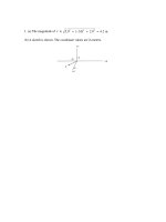
q
F = m1a1 = k 1 2 2 = 8.99 × 109
.
r

0.0032 2

c

h

Inserting the values for m1 and a1 (see part (a)) we obtain |q| = 7.1 × 10–11 C.


2. The magnitude of the mutual force of attraction at r = 0.120 m is

hc

hc

h

3.00 × 10−6 150
. × 10−6
q1 q2
9
F=k
= 8.99 × 10
= 2.81 N .
r2
0120
. 2

c

3. Eq. 21-1 gives Coulomb’s Law, F = k
k | q1 || q2 |
r=
=
F

(8.99 ×10 N ⋅ m
9

2

q1 q2
r2

, which we solve for the distance:

C2 ) ( 26.0 ×10−6 C ) ( 47.0 ×10−6 C )
5.70N

= 1.39m.


4. The fact that the spheres are identical allows us to conclude that when two spheres are
in contact, they share equal charge. Therefore, when a charged sphere (q) touches an
uncharged one, they will (fairly quickly) each attain half that charge (q/2). We start with
spheres 1 and 2 each having charge q and experiencing a mutual repulsive force
F = kq 2 / r 2 . When the neutral sphere 3 touches sphere 1, sphere 1’s charge decreases to
q/2. Then sphere 3 (now carrying charge q/2) is brought into contact with sphere 2, a total
amount of q/2 + q becomes shared equally between them. Therefore, the charge of sphere

3 is 3q/4 in the final situation. The repulsive force between spheres 1 and 2 is finally
(q / 2)(3q / 4) 3 q 2 3
F' 3
F′ = k
= k 2= F Ÿ
= = 0.375.
2
r
F 8
8 r
8


5. The magnitude of the force of either of the charges on the other is given by

F=

b

1 q Q−q
r2
4 πε 0

g

where r is the distance between the charges. We want the value of q that maximizes the
function f(q) = q(Q – q). Setting the derivative df/dq equal to zero leads to Q – 2q = 0, or
q = Q/2. Thus, q/Q = 0.500.

6. For ease of presentation (of the computations below) we assume Q > 0 and q < 0
(although the final result does not depend on this particular choice).
(a) The x-component of the force experienced by q1 = Q is
§
·
Q )( Q )
| q |) ( Q ) ¸ Q | q | § Q / | q | ·
(
(
¨
F1x =
−
cos 45° +
2
2
¸ = 4πε a 2 ¨© − 2 2 + 1¸¹
a
4πε 0 ¨¨
0
¸
2a
©
¹
1

(

)

which (upon requiring F1x = 0) leads to Q / | q |= 2 2 , or Q / q = −2 2 = −2.83.

(b) The y-component of the net force on q2 = q is
§
·
| q |) ( Q ) ¸
(
1 ¨ | q |2
| q |2 § 1
Q·
F2 y =
sin
45
°
−
=
−
¨
2
2
2
¸ 4πε a © 2 2 | q | ¸¹
4πε 0 ¨¨ 2a
a
0
¸
©
¹

(

)

which (if we demand F2y = 0) leads to Q / q = −1/ 2 2 . The result is inconsistent with
that obtained in part (a). Thus, we are unable to construct an equilibrium configuration
with this geometry, where the only forces present are given by Eq. 21-1.


7. The force experienced by q3 is
G G
G
G
| q || q | ·
1 § | q3 || q1 | ˆ | q3 || q2 |
F3 = F31 + F32 + F34 =
j+
(cos45°ˆi + sin 45°ˆj) + 3 2 4 ˆi ¸
¨−
2
2
a
a
4πε 0 ©
( 2a )
¹

(a) Therefore, the x-component of the resultant force on q3 is
2 (1.0 ×10−7 ) § 1
| q3 | § | q2 |
·
·

9
F3 x =
+ | q4 | ¸ = ( 8.99 ×10 )
+ 2 ¸ = 0.17N.
¨
2 ¨
2
4πε 0 a © 2 2
(0.050)
¹
©2 2
¹
2

(b) Similarly, the y-component of the net force on q3 is
2 (1.0 ×10−7 ) §
| q3 | §
| q2 | ·
1 ·
9
F3 y =
− | q1 | +
= ( 8.99 ×10 )
−1 +
¸
¨
¸ = −0.046N.
2 ¨
2
4πε 0 a ©

(0.050)
2 2¹
2 2¹
©
2


8. (a) The individual force magnitudes (acting on Q) are, by Eq. 21-1,
k

q1 Q

b−a − g

a 2
2

=k

q2 Q

ba − g

a 2
2

which leads to |q1| = 9.0 |q2|. Since Q is located between q1 and q2, we conclude q1 and q2
are like-sign. Consequently, q1/q2 = 9.0.
(b) Now we have
k

q1 Q

b−a − g

3a 2
2

=k

q2 Q

ba − g

3a 2
2

which yields |q1| = 25 |q2|. Now, Q is not located between q1 and q2, one of them must
push and the other must pull. Thus, they are unlike-sign, so q1/q2 = –25.


9. We assume the spheres are far apart. Then the charge distribution on each of them is
spherically symmetric and Coulomb’s law can be used. Let q1 and q2 be the original
charges. We choose the coordinate system so the force on q2 is positive if it is repelled by
q1. Then, the force on q2 is
Fa = −

1 q1q2
qq
= −k 1 2 2

2
4 πε 0 r
r

where r = 0.500 m. The negative sign indicates that the spheres attract each other. After
the wire is connected, the spheres, being identical, acquire the same charge. Since charge
is conserved, the total charge is the same as it was originally. This means the charge on
each sphere is (q1 + q2)/2. The force is now one of repulsion and is given by
1
Fb =
4 πε 0

q1 + q2
2

q1 + q2
2

d id i = k bq + q g .
2

1

r2

2

4r 2

We solve the two force equations simultaneously for q1 and q2. The first gives the product

b

gb

g

2

0.500 m 0108
.
N
r 2 Fa
q1q2 = −
=−
= −3.00 × 10−12 C 2 ,
9
2
k
8.99 × 10 N ⋅ m C 2
and the second gives the sum
q1 + q2 = 2r

Fb
= 2 0.500 m
k

b

g

0.0360 N
= 2.00 × 10−6 C
9
2
2
8.99 × 10 N ⋅ m C

where we have taken the positive root (which amounts to assuming q1 + q2 ≥ 0). Thus, the
product result provides the relation
q2 =

− ( 3.00 ×10−12 C2 )
q1

which we substitute into the sum result, producing
q1 −

3.00 × 10−12 C 2
= 2.00 × 10−6 C.
q1

Multiplying by q1 and rearranging, we obtain a quadratic equation


c

h

q12 − 2.00 × 10−6 C q1 − 3.00 × 10−12 C 2 = 0 .

The solutions are

q1 =

2.00 × 10−6 C ±

2

c−2.00 × 10 Ch − 4c−3.00 × 10
−6

2

−12

C2

h.

If the positive sign is used, q1 = 3.00 × 10–6 C, and if the negative sign is used,
q1 = −1.00 ×10−6 C .
(a) Using q2 = (–3.00 × 10–12)/q1 with q1 = 3.00 × 10–6 C, we get q2 = −1.00 ×10−6 C .
(b) If we instead work with the q1 = –1.00 × 10–6 C root, then we find q2 = 3.00 ×10−6 C .
Note that since the spheres are identical, the solutions are essentially the same: one sphere
originally had charge –1.00 × 10–6 C and the other had charge +3.00 × 10–6 C.
What if we had not made the assumption, above, that q1 + q2 ≥ 0? If the signs of the
charges were reversed (so q1 + q2 < 0), then the forces remain the same, so a charge of
+1.00 × 10–6 C on one sphere and a charge of –3.00 × 10–6 C on the other also satisfies
the conditions of the problem.

10. With rightwards positive, the net force on q3 is
F3 = F13 + F23 = k

q1q3

( L12 + L23 )

2

+k

q2 q3
.
L223

We note that each term exhibits the proper sign (positive for rightward, negative for
leftward) for all possible signs of the charges. For example, the first term (the force
exerted on q3 by q1) is negative if they are unlike charges, indicating that q3 is being
pulled toward q1, and it is positive if they are like charges (so q3 would be repelled from
q1). Setting the net force equal to zero L23= L12 and canceling k, q3 and L12 leads to
q1
q
+ q2 = 0 Ÿ 1 = −4.00.
4.00
q2


11. (a) Eq. 21-1 gives

( 20.0 ×10 C ) = 1.60N.
qq
F12 = k 1 22 = ( 8.99 ×109 N ⋅ m 2 C2 )
2
d
(1.50m )
−6

2

(b) A force diagram is shown as well as our choice of y axis (the dashed line).

The y axis is meant to bisect the line between q2 and q3 in order to make use of the
symmetry in the problem (equilateral triangle of side length d, equal-magnitude charges
q1 = q2 = q3 = q). We see that the resultant force is along this symmetry axis, and we
obtain

F qI
= 2 G k J cos 30° = 2.77 N .
H dK
2

Fy

2


12. (a) According to the graph, when q3 is very close to q1 (at which point we can
consider the force exerted by particle 1 on 3 to dominate) there is a (large) force in the

positive x direction. This is a repulsive force, then, so we conclude q1 has the same sign
as q3. Thus, q3 is a positive-valued charge.
(b) Since the graph crosses zero and particle 3 is between the others, q1 must have the
same sign as q2, which means it is also positive-valued. We note that it crosses zero at r
= 0.020 m (which is a distance d = 0.060 m from q2). Using Coulomb’s law at that point,
we have
q3 q2
q1 q3
=
4πεo r2 4πεo d2
or q2/q1 = 9.0.

2

Ÿ

d
q2 = §¨ 2 ·¸ q1 = 9.0 q1 ,
©r ¹


13. (a) There is no equilibrium position for q3 between the two fixed charges, because it is
being pulled by one and pushed by the other (since q1 and q2 have different signs); in this
region this means the two force arrows on q3 are in the same direction and cannot cancel.
It should also be clear that off-axis (with the axis defined as that which passes through the
two fixed charges) there are no equilibrium positions. On the semi-infinite region of the
axis which is nearest q2 and furthest from q1 an equilibrium position for q3 cannot be
found because |q1| < |q2| and the magnitude of force exerted by q2 is everywhere (in that
region) stronger than that exerted by q1 on q3. Thus, we must look in the semi-infinite
region of the axis which is nearest q1 and furthest from q2, where the net force on q3 has

magnitude
k

q1q3
q2 q3
−k
2
x
d+x

b

g

2

with d = 10 cm and x assumed positive. We set this equal to zero, as required by the
problem, and cancel k and q3. Thus, we obtain
q1
q2
−
2
x
d+x

b

F d + x IJ
= 0ŸG
H x K

g
2

2

=

q2
=3
q1

which yields (after taking the square root)
d+x
d
= 3Ÿx=
≈ 14 cm
x
3 −1

for the distance between q3 and q1.
(b) As stated above, y = 0.


14. Since the forces involved are proportional to q, we see that the essential difference
between the two situations is Fa ∝ qB + qC (when those two charges are on the same side)
versus Fb ∝ −qB + qC (when they are on opposite sides). Setting up ratios, we have
qB + qC
Fa
=
Fb

- qB + qC

Ÿ

20.14
1+r
=
-2.877
-1 + r

where in the last step we have canceled (on the left hand side) 10−24 N from the numerator
and the denominator, and (on the right hand side) introduced the symbol r = qC /qB .
After noting that the ratio on the left hand side is very close to – 7, then, after a couple of
algebra steps, we are led to

r=

7 +1 8
= = 1.333.
7 −1 6


15. (a) The distance between q1 and q2 is
r12 =

( x2 − x1 ) + ( y2 − y1 )
2

2

=

( −0.020 − 0.035) + ( 0.015 − 0.005)
2

2

= 0.056 m.

The magnitude of the force exerted by q1 on q2 is
| q q | ( 8.99 ×10
F21 = k 1 2 2 =
r12

9

) ( 3.0 ×10 ) ( 4.0 ×10 ) = 35 N.
−6

−6

(0.056) 2

G
(b) The vector F21 is directed towards q1 and makes an angle θ with the +x axis, where
§ y2 − y1 ·
−1 § 1.5 − 0.5 ·
¸ = tan ¨
¸ = −10.3° ≈ −10°.
© −2.0 − 3.5 ¹

© x2 − x1 ¹

θ = tan −1 ¨

(c) Let the third charge be located at (x3, y3), a distance r from q2. We note that q1, q2 and
q3 must be collinear; otherwise, an equilibrium position for any one of them would be
impossible to find. Furthermore, we cannot place q3 on the same side of q2 where we also
find q1, since in that region both forces (exerted on q2 by q3 and q1) would be in the same
direction (since q2 is attracted to both of them). Thus, in terms of the angle found in part
(a), we have x3 = x2 – r cosθ and y3 = y2 – r sinθ (which means y3 > y2 since θ is negative).
The magnitude of force exerted on q2 by q3 is F23 = k | q2 q3 | r 2 , which must equal that of
the force exerted on it by q1 (found in part (a)). Therefore,
k

q2 q3
qq
q
= k 1 2 2 Ÿ r = r12 3 = 0.0645 cm .
2
r
r12
q1

Consequently, x3 = x2 – r cosθ = –2.0 cm – (6.45 cm) cos(–10°) = –8.4 cm,
(d) and y3 = y2 – r sinθ = 1.5 cm – (6.45 cm) sin(–10°) = 2.7 cm.


16. (a) For the net force to be in the +x direction, the y components of the individual
forces must cancel. The angle of the force exerted by the q1 = 40 µC charge on
q3 = 20 µ C is 45°, and the angle of force exerted on q3 by Q is at –θ where

θ = tan −1

FG 2.0IJ = 33.7° .
H 3.0 K

Therefore, cancellation of y components requires
k

q1 q3

( 0.02 2 )

2

sin 45° = k

(

| Q | q3
(0.030) + (0.020)
2

2

)

2

sin θ

from which we obtain |Q| = 83 µC. Charge Q is “pulling” on q3, so (since q3 > 0) we
conclude Q = –83 µC.
(b) Now, we require that the x components cancel, and we note that in this case, the angle
of force on q3 exerted by Q is +θ (it is repulsive, and Q is positive-valued). Therefore,
k

q1 q3

( 0.02 2 )

2

cos 45° = k

(

Qq3
(0.030) + (0.020)

from which we obtain Q = 55.2 µC ≈ 55 µ C .

2

2

)

2

cos θ


17. (a) If the system of three charges is to be in equilibrium, the force on each charge
must be zero. The third charge q3 must lie between the other two or else the forces acting
on it due to the other charges would be in the same direction and q3 could not be in
equilibrium. Suppose q3 is at a distance x from q, and L – x from 4.00q. The force acting
on it is then given by
F3 =

4qq3 ·
1 § qq3
¨ 2 −
¸
2
4πε 0 ¨© x
( L − x ) ¸¹

where the positive direction is rightward. We require F3 = 0 and solve for x. Canceling
common factors yields 1/x2 = 4/(L – x)2 and taking the square root yields 1/x = 2/(L – x).
The solution is x = L/3.
The force on q is
Fq =

−1 § qq3 4.00q 2 ·
+
¨
¸.
L2 ¹
4 πε 0 © x 2

The signs are chosen so that a negative force value would cause q to move leftward. We
require Fq = 0 and solve for q3:
q3 = −

q
4qx 2
4
4
= − q Ÿ 3 = − = −0.444
2
L
9
q
9

where x = L/3 is used. We may easily verify that the force on 4.00q also vanishes:
F4 q =

2
4qq0 ·
1 § 4q 2
1 § 4q 2 4 ( − 4 9 ) q ·
1 § 4q 2 4q 2 ·
=
+
=
−
=0.
¨ 2 +

¸
¨
¸
2
4πε 0 ¨© L
( 4 9 ) L2 ¸¹ 4πε 0 ¨© L2 L2 ¸¹
( L − x ) ¸¹ 4πε 0 ¨© L2

(b) As seen above, q3 is located at x = L/3. With L = 9.00 cm, we have x = 3.00 cm.
(c) Similarly, the y coordinate of q3 is y = 0.


1

18. (a) We note that cos(30º) = 2 3 , so that the dashed line distance in the figure is
r = 2d / 3 . We net force on q1 due to the two charges q3 and q4 (with |q3| = |q4| = 1.60 ×
10−19 C) on the y axis has magnitude

2

| q1q3 |
3 3 | q1q3 |
cos(30°) =
.
2
4πε 0 r
16πε 0 d 2

This must be set equal to the magnitude of the force exerted on q1 by q2 = 8.00 × 10−19 C
= 5.00 |q3| in order that its net force be zero:

3 3 | q1q3 |
| q1q2 |
=
2
16πε 0 d
4πε 0 ( D + d ) 2

Ÿ

§
D = d ¨2
©

·
− 1¸ = 0.9245 d .
3 3
¹
5

Given d = 2.00 cm, then this leads to D = 1.92 cm.
(b) As the angle decreases, its cosine increases, resulting in a larger contribution from the
charges on the y axis. To offset this, the force exerted by q2 must be made stronger, so
that it must be brought closer to q1 (keep in mind that Coulomb’s law is inversely
proportional to distance-squared). Thus, D must be decreased.


19. The charge dq within a thin shell of thickness dr is ρ A dr where A = 4πr2. Thus, with
ρ = b/r, we have

z

q = dq = 4 πb

z

r2

r1

c

h

r dr = 2πb r22 − r12 .

With b = 3.0 µC/m2, r2 = 0.06 m and r1 = 0.04 m, we obtain q = 0.038 µC = 3.8 × 10−8 C.


20. If θ is the angle between the force and the x-axis, then
cosθ =

x
.
x + d2
2

We note that, due to the symmetry in the problem, there is no y component to the net
force on the third particle. Thus, F represents the magnitude of force exerted by q1 or q2
on q3. Let e = +1.60 × 10−19 C, then q1 = q2 = +2e and q3 = 4.0e and we have
Fnet = 2F cosθ =

2(2e)(4e)
4πεo (x2 + d2)

4e2 x
x
=
.
πεo (x2 + d2 )3/2
x2 + d2

(a) To find where the force is at an extremum, we can set the derivative of this expression
equal to zero and solve for x, but it is good in any case to graph the function for a fuller
understanding of its behavior – and as a quick way to see whether an extremum point is a
maximum or a miminum. In this way, we find that the value coming from the derivative
procedure is a maximum (and will be presented in part (b)) and that the minimum is
found at the lower limit of the interval. Thus, the net force is found to be zero at x = 0,
which is the smallest value of the net force in the interval 5.0 m ≥ x ≥ 0.
(b) The maximum is found to be at x = d/ 2 or roughly 12 cm.
(c) The value of the net force at x = 0 is Fnet = 0.
(d) The value of the net force at x = d/ 2 is Fnet = 4.9 × 10−26 N.


21. (a) The magnitude of the force between the (positive) ions is given by

bqgbqg = k q
F=
4 πε 0r 2

2

r2

where q is the charge on either of them and r is the distance between them. We solve for
the charge:
q=r

F
= 5.0 × 10−10 m
k

c

h

3.7 × 10−9 N
= 3.2 × 10−19 C.
9
2
2
8.99 × 10 N ⋅ m C

(b) Let N be the number of electrons missing from each ion. Then, Ne = q, or
N=

q 3.2 × 10−9 C
=
= 2.
. × 10−19 C
e 16

22. The magnitude of the force is

FG
H

e2
N ⋅ m2
F = k 2 = 8.99 × 109
r
C2

−19

2

−10

2

. × 10 Ch
IJ c160
K c2.82 × 10 mh

= 2.89 × 10−9 N .


23. Eq. 21-11 (in absolute value) gives
q 10

. × 10−7 C
n= =
= 6.3 × 1011 .
−19
. × 10 C
e 16


24. (a) Eq. 21-1 gives
. × 10 Ch
c8.99 × 10 N ⋅ m C hc100
F=
. × 10 mh
c100
9

2

−16

2

−2

2

2

= 8.99 × 10−19 N .

(b) If n is the number of excess electrons (of charge –e each) on each drop then
n=−

. × 10−16 C
q
−100
=−
= 625.
160
. × 10−19 C
e