Solution manual fundamentals of physics extended, 8th editionch26

1. (a) The charge that passes through any cross section is the product of the current and
time. Since 4.0 min = (4.0 min)(60 s/min) = 240 s, q = it = (5.0 A)(240 s) = 1.2× 103 C.
(b) The number of electrons N is given by q = Ne, where e is the magnitude of the charge
on an electron. Thus,
N = q/e = (1200 C)/(1.60 × 10–19 C) = 7.5 × 1021.


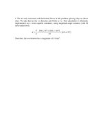
2. We adapt the discussion in the text to a moving two-dimensional collection of charges.
Using σ for the charge per unit area and w for the belt width, we can see that the transport
of charge is expressed in the relationship i = σvw, which leads to

σ=

i
100 × 10−6 A
2
=
= 6.7 × 10−6 C m .
−2
vw
30 m s 50 × 10 m

b

gc

h


3. Suppose the charge on the sphere increases by ∆q in time ∆t. Then, in that time its
potential increases by

∆V =

∆q
,
4 πε 0 r

where r is the radius of the sphere. This means
∆q = 4 πε 0 r ∆V .

Now, ∆q = (iin – iout) ∆t, where iin is the current entering the sphere and iout is the current
leaving. Thus,

∆t =
=

∆q
4 πε 0 r ∆V
=
iin − iout
iin − iout

c8.99 × 10

9

. mgb1000 Vg
b010
= 5.6 × 10
F / mh b10000020
.

A − 10000000
.
Ag

−3

s.


4. We express the magnitude of the current density vector in SI units by converting the
diameter values in mils to inches (by dividing by 1000) and then converting to meters (by
multiplying by 0.0254) and finally using
J=

4i
i
i
.
=
=
2
A πR
πD 2

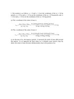
For example, the gauge 14 wire with D = 64 mil = 0.0016 m is found to have a
(maximum safe) current density of J = 7.2 × 106 A/m2. In fact, this is the wire with the
largest value of J allowed by the given data. The values of J in SI units are plotted below
as a function of their diameters in mils.

5. (a) The magnitude of the current density is given by J = nqvd, where n is the number of
particles per unit volume, q is the charge on each particle, and vd is the drift speed of the
particles. The particle concentration is n = 2.0 × 108/cm3 = 2.0 × 1014 m–3, the charge is
q = 2e = 2(1.60 × 10–19 C) = 3.20 × 10–19 C,
and the drift speed is 1.0 × 105 m/s. Thus,

c

hc

hc

h

J = 2 × 1014 / m 3.2 × 10−19 C 10
. × 105 m / s = 6.4 A / m2 .

(b) Since the particles are positively charged the current density is in the same direction
as their motion, to the north.
(c) The current cannot be calculated unless the cross-sectional area of the beam is known.
Then i = JA can be used.


6. (a) The magnitude of the current density vector is

c
c

h
h

4 12
. × 10−10 A
i
i
J= =
=
= 2.4 × 10−5 A / m2 .
2
2
−
3
A πd / 4 π 2.5 × 10 m
(b) The drift speed of the current-carrying electrons is
vd =

J
2.4 × 10−5 A / m2
=
= 18
. × 10−15 m / s.
ne 8.47 × 1028 / m3 160
. × 10−19 C

c

hc

h

7. The cross-sectional area of wire is given by A = πr2, where r is its radius (half its
thickness). The magnitude of the current density vector is J = i / A = i / πr 2 , so

r=

i
=
πJ

0.50 A
. × 10−4 m.
= 19
4
2
π 440 × 10 A / m

c

h

The diameter of the wire is therefore d = 2r = 2(1.9 × 10–4 m) = 3.8 × 10–4 m.


8. (a) Since 1 cm3 = 10–6 m3, the magnitude of the current density vector is

J = nev =

FG 8.70 IJ c160
H 10 m K . × 10 Chc470 × 10 m / sh = 6.54 × 10

−19

−6

3

3

−7

A / m2 .

(b) Although the total surface area of Earth is 4 πRE2 (that of a sphere), the area to be used
in a computation of how many protons in an approximately unidirectional beam (the solar
wind) will be captured by Earth is its projected area. In other words, for the beam, the
encounter is with a “target” of circular area πRE2 . The rate of charge transport implied by
the influx of protons is

c

h c6.54 × 10

i = AJ = πRE2 J = π 6.37 × 106 m

2

−7

h

A / m2 = 8.34 × 107 A.


9. We use vd = J/ne = i/Ane. Thus,
−14
2
28
3
−19
L
L
LAne ( 0.85m ) ( 0.21× 10 m ) ( 8.47 ×10 / m ) (1.60 ×10 C )
=
=
=
t=
vd i / Ane
i
300A

= 8.1×102 s = 13min .


10. We note that the radial width ∆r = 10 µm is small enough (compared to r = 1.20 mm)
that we can make the approximation
´
¶

Br 2πr dr ≈ Br 2πr ∆r .

Thus, the enclosed current is 2πBr2∆r = 18.1 µA. Performing the integral gives the same
answer.


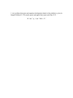
11. (a) The current resulting from this non-uniform current density is
i=³

cylinder

J a dA =

J0
R

³

R

0

2
2
r ⋅ 2π rdr = π R 2 J 0 = π (3.40 ×10−3 m) 2 (5.50 ×104 A/m 2 ) = 1.33 A .
3
3

(b) In this case,
R
1
1

§ r·
J b dA = ³ J 0 ¨1 − ¸ 2π rdr = π R 2 J 0 = π (3.40 ×10−3 m) 2 (5.50 ×104 A/m 2 )
cylinder
0
3
3
© R¹
= 0.666 A.

i=³

(c) The result is different from that in part (a) because Jb is higher near the center of the
cylinder (where the area is smaller for the same radial interval) and lower outward,
resulting in a lower average current density over the cross section and consequently a
lower current than that in part (a). So, Ja has its maximum value near the surface of the
wire.


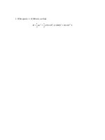
G
12. Assuming J is directed along the wire (with no radial flow) we integrate, starting
with Eq. 26-4,
G
R
i = ³ | J | dA = ³

1
(kr 2 )2πrdr = k π ( R 4 − 0.656 R 4 )
9 R /10
2

where k = 3.0 × 108 and SI units understood. Therefore, if R = 0.00200 m, we
obtain i = 2.59 ×10−3 A .


13. We find the conductivity of Nichrome (the reciprocal of its resistivity) as follows:

σ=

1

ρ

=

b

gb

g

10
. m 4.0 A
L
L
Li
=
=
=
= 2.0 × 106 / Ω ⋅ m.
−6

2
RA V / i A VA
. × 10 m
2.0 V 10

b g

b

gc

h


14. We use R/L = ρ/A = 0.150 Ω/km.
(a) For copper J = i/A = (60.0 A)(0.150 Ω/km)/(1.69 × 10–8 Ω·m) = 5.32 × 105 A/m2.
(b) We denote the mass densities as ρm. For copper,
(m/L)c = (ρmA)c = (8960 kg/m3) (1.69 × 10–8 Ω· m)/(0.150 Ω/km) = 1.01 kg/m.
(c) For aluminum J = (60.0 A)(0.150 Ω/km)/(2.75 × 10–8 Ω·m) = 3.27 × 105 A/m2.
(d) The mass density of aluminum is
(m/L)a = (ρmA)a = (2700 kg/m3)(2.75 × 10–8 Ω·m)/(0.150 Ω/km) = 0.495 kg/m.


15. The resistance of the wire is given by R = ρL / A , where ρ is the resistivity of the
material, L is the length of the wire, and A is its cross-sectional area. In this case,

c

h

2

A = πr 2 = π 0.50 × 10−3 m = 7.85 × 10−7 m2 .
Thus,
−3
−7
2
RA ( 50 ×10 Ω ) ( 7.85 ×10 m )
ρ=
=
= 2.0 ×10−8 Ω⋅ m.
L
2.0m


16. (a) i = V/R = 23.0 V/15.0 × 10–3 Ω = 1.53 × 103 A.
(b) The cross-sectional area is A = πr 2 = 41 πD 2 . Thus, the magnitude of the current
density vector is

c

h
h

. × 10−3 A
4 153
4i
i
J= =
=

A πD 2 π 6.00 × 10−3 m

c

2

= 5.41 × 107 A / m2 .

(c) The resistivity is

c

hb gc

h

2

ρ = RA / L = 15.0 × 10−3 Ω π 6.00 × 103 m / [4(4.00 m)] = 10.6 × 10−8 Ω ⋅ m.
(d) The material is platinum.


17. Since the potential difference V and current i are related by V = iR, where R is the
resistance of the electrician, the fatal voltage is V = (50 × 10–3 A)(2000 Ω) = 100 V.


18. The thickness (diameter) of the wire is denoted by D. We use R ∝ L/A (Eq. 26-16)
and note that A = 41 πD 2 ∝ D 2 . The resistance of the second wire is given by

F A IF L I F D I F L I

F 1I
= RG J G J = RG J G J = Rb2g G J = 2 R.
H 2K
H A KH L K HD K H L K
2

R2

1

2

1

2

2

1

2

1

2


19. The resistance of the coil is given by R = ρL/A, where L is the length of the wire, ρ is
the resistivity of copper, and A is the cross-sectional area of the wire. Since each turn of
wire has length 2πr, where r is the radius of the coil, then

L = (250)2πr = (250)(2π)(0.12 m) = 188.5 m.
If rw is the radius of the wire itself, then its cross-sectional area is A = πr2w = π(0.65 ×
10–3 m)2 = 1.33 × 10–6 m2. According to Table 26-1, the resistivity of copper is
. × 10−8 Ω ⋅ m . Thus,
169
R=

ρL
A

=

. × 10
c169

−8

hb

g = 2.4 Ω.

Ω ⋅ m 188.5 m

133
. × 10

−6

m

2


20. (a) Since the material is the same, the resistivity ρ is the same, which implies (by Eq.
26-11) that the electric fields (in the various rods) are directly proportional to their
current-densities. Thus, J1: J2: J3 are in the ratio 2.5/4/1.5 (see Fig. 26-24). Now the
currents in the rods must be the same (they are “in series”) so
J1 A1 = J3 A3

and

J2 A2 = J3 A3 .

Since A = πr2 this leads (in view of the aforementioned ratios) to
4r22 = 1.5r32

and

2.5r12 = 1.5r32 .

Thus, with r3 = 2 mm, the latter relation leads to r1 = 1.55 mm.
(b) The 4r22 = 1.5r32 relation leads to r2 = 1.22 mm.


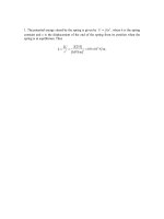
21. Since the mass density of the material do not change, the volume remains the same. If
L0 is the original length, L is the new length, A0 is the original cross-sectional area, and A
is the new cross-sectional area, then L0A0 = LA and A = L0A0/L = L0A0/3L0 = A0/3. The
new resistance is
R=

ρL
A

=

ρ 3 L0
A0 / 3

=9

ρL0
A0

= 9 R0 ,

where R0 is the original resistance. Thus, R = 9(6.0 Ω) = 54 Ω.


22. The cross-sectional area is A = πr2 = π(0.002 m)2. The resistivity from Table 26-1 is
ρ = 1.69 × 10−8 Ω·m. Thus, with L = 3 m, Ohm’s Law leads to V = iR = iρL/A, or
12 × 10−6 V = i (1.69 × 10−8 Ω·m)(3.0 m)/ π(0.002 m)2
which yields i = 0.00297 A or roughly 3.0 mA.


23. The resistance of conductor A is given by
RA =

ρL
πrA2

,

where rA is the radius of the conductor. If ro is the outside diameter of conductor B and ri
is its inside diameter, then its cross-sectional area is π(ro2 – ri2), and its resistance is
RB =

c

ρL

π ro2 − ri 2

h.

The ratio is

b

g b
2

g

1.0 mm − 0.50 mm
R A ro2 − ri 2
=
=
2
2
RB

rA
0.50 mm

b

g

2

= 3.0.


24. The absolute values of the slopes (for the straight-line segments shown in the graph of
Fig. 26-26(b)) are equal to the respective electric field magnitudes. Thus, applying Eq.
26-5 and Eq. 26-13 to the three sections of the resistive strip, we have
i
J1 = A = σ1 E1 = σ1 (0.50 × 103 V/m)
i
J2 = A = σ2 E2 = σ2 (4.0 × 103 V/m)
i
J3 = A = σ3 E3 = σ3 (1.0 × 103 V/m) .
We note that the current densities are the same since the values of i and A are the same
(see the problem statement) in the three sections, so J1 = J2 = J3 .
(a) Thus we see that
σ1 = 2σ3 = 2 (3.00 × 107(Ω·m)−1 ) = 6.00 × 107 (Ω·m)−1.
(b) Similarly, σ2 = σ3/4 = (3.00 × 107(Ω·m)−1 )/4 = 7.50 × 106 (Ω·m)−1 .


25. The resistance at operating temperature T is R = V/i = 2.9 V/0.30 A = 9.67 Ω. Thus,
from R – R0 = R0α (T – T0), we find

T = T0 +

§
· § 9.67 Ω ·
1 § R ·
1
− 1¸ = 1.9 ×103 °C .
¨ −1¸ = 20°C + ¨
¸¨
−3
α © R0 ¹
© 4.5 ×10 K ¹ © 1.1Ω
¹

Since a change in Celsius is equivalent to a change on the Kelvin temperature scale, the
value of α used in this calculation is not inconsistent with the other units involved. Table
26-1 has been used.