Solution manual vector mechanics engineers dynamics 8th beer chapter 09
Bạn đang xem bản rút gọn của tài liệu. Xem và tải ngay bản đầy đủ của tài liệu tại đây (22.18 MB, 290 trang )
COSMOS: Complete Online Solutions Manual Organization System
Chapter 9, Solution 1.
First note:
Have
y=
b2 − b1
x + b1
a
I y = ∫ x 2dA
b2 − b1
x + b1
a
a
x 2d ydx
0 0
=∫ ∫
a
b − b1
= ∫ 0 x2 2
x + b1 dx
a
a
1 b − b1 4 1 3
= 2
x + b1x
3
4 a
0
=
1 3
a ( b1 + 3b2 )
12
Iy =
Vector Mechanics for Engineers: Statics and Dynamics, 8/e, Ferdinand P. Beer, E. Russell Johnston, Jr.,
Elliot R. Eisenberg, William E. Clausen, David Mazurek, Phillip J. Cornwell
© 2007 The McGraw-Hill Companies.
1 3
a ( b1 + 3b2 )
12
COSMOS: Complete Online Solutions Manual Organization System
Chapter 9, Solution 2.
At
5
x = a, y = b :
∴ y =
b
a
5
2
5
b = ka 2
x2
or
dI y =
1 3
x dy
3
=
Then
Iy =
x=
or
a
b
b
5
a2
2
2
5
y5
1 a3 65
y dy
3 b 65
1 a3 b 65
∫ y dy
3 b 65 0
1 5 a3 115
=
y
3 11 b 65
=
k =
b
0
5 a3 115
b
33 b 65
or I y =
Vector Mechanics for Engineers: Statics and Dynamics, 8/e, Ferdinand P. Beer, E. Russell Johnston, Jr.,
Elliot R. Eisenberg, William E. Clausen, David Mazurek, Phillip J. Cornwell
© 2007 The McGraw-Hill Companies.
5 3
ab
33
COSMOS: Complete Online Solutions Manual Organization System
Chapter 9, Solution 3.
At x = 0:
First note:
At x = a :
a = k ( 2b − b )
k =
∴ x=
Have
2
c = −b
or
or
0 = k (b + c)
2
a
b2
a
2
y − b)
2(
b
I y = ∫ x 2dA
=∫
a
2
y − b)
2b b 2 (
0
0
∫
x 2dxdy
3
=
1 2b a
2
y − b ) dy
∫
0 2(
3
b
2b
1 a3 1
7
=
× ( y − b)
6
3b
7
b
=
1 3
ab
21
Iy =
Vector Mechanics for Engineers: Statics and Dynamics, 8/e, Ferdinand P. Beer, E. Russell Johnston, Jr.,
Elliot R. Eisenberg, William E. Clausen, David Mazurek, Phillip J. Cornwell
© 2007 The McGraw-Hill Companies.
1 3
ab
21
COSMOS: Complete Online Solutions Manual Organization System
Chapter 9, Solution 4.
y = kx 2 + c
Have
b = k ( 0) + c
x = 0, y = b :
At
c=b
or
At
x = 2a, y = 0:
or
k =−
y =−
Then
=
Then
I y = ∫ x 2dA,
2a
I y = ∫ a x 2dA =
2
0 = k ( 2a ) + b
b
4a 2
b 2
x +b
4a 2
b
4a 2 − x 2
4a 2
(
dA = ydx =
)
(
)
b
4a 2 − x 2 dx
4a 2
(
)
b 2a 2
2
2
∫ x 4a − x dx
4a 2 a
2a
b 2 x3 x5
=
−
4a
3
5 a
4a 2
=
b
b
8a3 − a3 −
32a5 − a5
2
3
20a
=
7a3b 31a3b
−
3
20
(
)
(
)
Iy =
Vector Mechanics for Engineers: Statics and Dynamics, 8/e, Ferdinand P. Beer, E. Russell Johnston, Jr.,
Elliot R. Eisenberg, William E. Clausen, David Mazurek, Phillip J. Cornwell
© 2007 The McGraw-Hill Companies.
47 3
ab
60
COSMOS: Complete Online Solutions Manual Organization System
Chapter 9, Solution 5.
First note:
Have
y =
b2 − b1
x + b1
a
I x = ∫ y 2dA
=
b2 − b1
x + b1
a
a
0 0
∫ ∫
y 2d ydx
3
1 a b − b1
= ∫0 2
x + b1 dx
3 a
4
1 1 a b2 − b1
= ×
x + b1
3 4 b2 − b1 a
a
0
=
1
a
b24 − b14
12 b2 − b1
=
1
a
( b2 + b1 )( b2 − b1 ) b22 + b12
12 b2 − b1
=
1
a ( b1 + b2 ) b12 + b22
12
(
)
(
(
)
)
Ix =
Vector Mechanics for Engineers: Statics and Dynamics, 8/e, Ferdinand P. Beer, E. Russell Johnston, Jr.,
Elliot R. Eisenberg, William E. Clausen, David Mazurek, Phillip J. Cornwell
© 2007 The McGraw-Hill Companies.
1
a ( b1 + b2 ) b12 + b22
12
(
)
COSMOS: Complete Online Solutions Manual Organization System
Chapter 9, Solution 6.
SOLUTION
5
At x = a, y = b : b = ka 2
or k =
∴y =
b
5
a2
b
a
5
x2
5
2
I x = ∫ y 2dA
=
b
a
2
y 5 dy
b
2
∫0 y
a
dA = xdy
2
5
5 175
= 2 ×
y
b 5 17
b
0
17
5a b 5
=
17 b 52
or I x =
Vector Mechanics for Engineers: Statics and Dynamics, 8/e, Ferdinand P. Beer, E. Russell Johnston, Jr.,
Elliot R. Eisenberg, William E. Clausen, David Mazurek, Phillip J. Cornwell
© 2007 The McGraw-Hill Companies.
5 3
ab
17
COSMOS: Complete Online Solutions Manual Organization System
Chapter 9, Solution 7.
At x = 0: 0 = k ( b + c )
First note:
or
2
c = −b
At x = a : a = k ( 2b − b )
Have
or
k =
a
b2
∴
x=
a
2
y − b)
2(
b
2
I x = ∫ y 2dA
=∫
a
2
y − b)
2b b 2 (
0
b
∫
y 2dxdy
=
a 2b 2
2
y ( y − b ) dy
2 ∫b
b
=
a 2b 4
y − 2by 3 + b 2 y 2 dy
2 ∫b
b
=
a 1 5 1 4 1 2 3
y − by + b y
2
3
b2 5
b
=
a 1
1
1 2
1 2 3
5
4
3
1 5 1
4
( 2b ) − ( 2b ) + b ( 2b ) − b − b b + b b
2
3
5
2
3
b 2 5
(
)
2b
( )
( )
8 1 1 1
32
= ab3
−8+ − + −
3 5 2 3
5
=
31 3
ab
30
Ix =
Vector Mechanics for Engineers: Statics and Dynamics, 8/e, Ferdinand P. Beer, E. Russell Johnston, Jr.,
Elliot R. Eisenberg, William E. Clausen, David Mazurek, Phillip J. Cornwell
© 2007 The McGraw-Hill Companies.
31 3
ab
30
COSMOS: Complete Online Solutions Manual Organization System
Chapter 9, Solution 8.
Have
y = kx 2 + c
At
x = 0, y = b: b = k (0) + c
or
c=b
At
x = 2a, y = 0: 0 = k (2a) 2 + b
or
k =−
Then
y =
Now
dI x =
=
b
4a 2
b
4a 2 − x 2
4a 2
(
)
1 3
y dx
3
3
1 b3
4a 2 − x 2 dx
6
3 64a
(
)
continued
Vector Mechanics for Engineers: Statics and Dynamics, 8/e, Ferdinand P. Beer, E. Russell Johnston, Jr.,
Elliot R. Eisenberg, William E. Clausen, David Mazurek, Phillip J. Cornwell
© 2007 The McGraw-Hill Companies.
COSMOS: Complete Online Solutions Manual Organization System
Then
I x = ∫ dI x
=
3
1 b3 2 a
4a 2 − x 2 dx
6 ∫a
3 64a
=
b3
2a
64a 6 − 48a 4 x 2 + 12a 2 x 4 − x 6 dx
6 ∫a
192a
(
)
(
)
2a
b3
12 2 5 x 7
6
4 3
64
a
x
16
a
x
a x −
=
−
+
5
7 a
192a 6
=
b3
64a 7( 2 − 1) − 16a 7 ( 8 − 1)
192a 6
+
=
12 7
1
a ( 32 − 1) − (128 − 1)
5
7
ab3
372 127
3
−
64 − 112 +
= 0.043006ab
192
5
7
I x = 0.0430ab3
Vector Mechanics for Engineers: Statics and Dynamics, 8/e, Ferdinand P. Beer, E. Russell Johnston, Jr.,
Elliot R. Eisenberg, William E. Clausen, David Mazurek, Phillip J. Cornwell
© 2007 The McGraw-Hill Companies.
COSMOS: Complete Online Solutions Manual Organization System
Chapter 9, Solution 9.
x2
y2
+
=1
a 2 b2
x = a 1−
y2
b2
dA = xdy
dI x = y 2dA = y 2 xdy
b
b
I x = ∫ dI x = ∫ − b xy 2dy = a ∫ − b y 2 1 −
Set: y = b sin θ
y2
dy
b2
dy = b cosθ dθ
π
I x = a ∫ 2π b 2 sin 2 θ 1 − sin 2 θ b cosθ dθ
−
2
π
π
−
−
= ab3 ∫ 2π sin 2 θ cos 2 θ dθ = ab3 ∫ 2π
2
2
1 2
sin 2θ dθ
4
π
π
1
1
1
1
2
= ab3 ∫ 2π (1 − cos 4θ ) dθ = ab3 θ − sin 4θ
− 2
4
8
4
−π
2
=
2
1 3 π π π 3
ab − − = ab
8
2 2 8
Vector Mechanics for Engineers: Statics and Dynamics, 8/e, Ferdinand P. Beer, E. Russell Johnston, Jr.,
Elliot R. Eisenberg, William E. Clausen, David Mazurek, Phillip J. Cornwell
© 2007 The McGraw-Hill Companies.
Ix =
1
π ab3
8
COSMOS: Complete Online Solutions Manual Organization System
Chapter 9, Solution 10.
At
2a = kb3
x = 2a, y = b:
or
k =
2a
b3
Then
x=
2a 3
y
b3
or
y =
Now
dI x =
b
( 2a )
1
1
3
x3
1 3
1 b3
y dx =
xdx
3
3 2a
2a
Then
1 b3 2 a
1 b3 1 2
I x = ∫ dI x =
xdx
x
=
∫
3 2a a
6 a 2 a
=
b3
4a 2 − a 2
12a
(
)
Ix =
Vector Mechanics for Engineers: Statics and Dynamics, 8/e, Ferdinand P. Beer, E. Russell Johnston, Jr.,
Elliot R. Eisenberg, William E. Clausen, David Mazurek, Phillip J. Cornwell
© 2007 The McGraw-Hill Companies.
1 3
ab
4
COSMOS: Complete Online Solutions Manual Organization System
Chapter 9, Solution 11.
−a
At x = a : b = k 1 − e a
First note:
or
Have
k =
b
1 − e−1
I x = ∫ y 2dA
b
a 1− e
0 0
=∫ ∫
−x
1− e a
−1
3
y 2dydx
3
=
−x
1 b a
1 − e a dx
−1 ∫ 0
31 − e
=
−x
−2 x
−3 x
1 b a
1 − 3e a + 3e a − e a dx
−1 ∫ 0
31 − e
3
3
a
−x
1 b
a −2 x a −3x
x − 3( − a ) e a + 3 − e a − − e a
=
−1
31 − e
2
3
0
3
1 b
1
1
=
a + 3ae−1 − 1.5ae−2 + ae −3 − 3a − 1.5a + a
−1
3 1 − e
3
3
=
1
ab3
3 1 − e −1
(
)
3
11
1.91723 −
6
= 0.1107ab3
I x = 0.1107ab3
Vector Mechanics for Engineers: Statics and Dynamics, 8/e, Ferdinand P. Beer, E. Russell Johnston, Jr.,
Elliot R. Eisenberg, William E. Clausen, David Mazurek, Phillip J. Cornwell
© 2007 The McGraw-Hill Companies.
COSMOS: Complete Online Solutions Manual Organization System
Chapter 9, Solution 12.
x2
y2
+
=1
a 2 b2
y = b 1−
x2
a2
dA = 2 ydx
dI y = x 2dA = 2 x 2 ydx
a
a
I y = ∫ dI y = ∫ 0 2 x 2 ydx = 2b ∫ 0 x 2 1 −
x = a sin θ
Set:
x2
dx
a2
dx = a cosθ dθ
π
I y = 2b∫ 02 a 2 sin 2 θ 1 − sin 2 θ a cosθ dθ
3
π
2
2
3
π
= 2a b∫ sin θ cos θ dθ = 2a b∫ 02
2
0
π
1 2
sin 2θ dθ
4
π
1
1
1
1
2
= a3b∫ 02 (1 − cos 4θ ) dθ = a3b θ − sin 4θ
2
2
4
4
0
=
1 3 π
π
a b − 0 = a3b
4
2
8
Iy =
Vector Mechanics for Engineers: Statics and Dynamics, 8/e, Ferdinand P. Beer, E. Russell Johnston, Jr.,
Elliot R. Eisenberg, William E. Clausen, David Mazurek, Phillip J. Cornwell
© 2007 The McGraw-Hill Companies.
1 3
πa b
8
COSMOS: Complete Online Solutions Manual Organization System
Chapter 9, Solution 13.
At
x = 2a, y = b : 2a = kb3
2a 3
y
b3
Then
x=
or
y =
Now
I y = ∫ x 2dA
Then
I y = ∫ a x2
b
( 2a )
=
=
=
1
b
( 2a )
1
3
x 3 dx
7
b
( 2a )
x3
dA = ydx
2a
=
1
1
3
1
3
b
1
( 2a ) 3
2a
∫ a x 3 dx
3 103
x
10
3b
10 ( 2a )
1
3
2a
a
2a 103 − a 103
( )
10
3ba3 103
2 − 1 3
1
10 ( 2 ) 3
= 2.1619a3b
or I y = 2.16a3b
Vector Mechanics for Engineers: Statics and Dynamics, 8/e, Ferdinand P. Beer, E. Russell Johnston, Jr.,
Elliot R. Eisenberg, William E. Clausen, David Mazurek, Phillip J. Cornwell
© 2007 The McGraw-Hill Companies.
COSMOS: Complete Online Solutions Manual Organization System
Chapter 9, Solution 14.
First note:
or
Have
−a
At x = a : b = k 1 − e a
k =
b
1 − e−1
I y = ∫ x 2dA
b
a 1− e
0 0
−x
1− e a
−1
2
x d ydx
=
∫ ∫
=
∫ 0 x 1 − e−1 1 − e a dx
a 2
b
−x
a
−x
2
b 1 3
e a 1 2
1
x
x
2
x
2
=
−
−
−
−
+
3
1 − e−1 3
a
1 a
−
a
0
=
2
b 1 3
a
3 −1 a
3
+
a
a
e
2 + 2 + 2 − a × 2
−1
a
1 − e 3
a
=
a3b 1
+ 5e −1 − 2
−1
1− e 3
(
)
= 0.273a3b
I y = 0.273 a3b
Vector Mechanics for Engineers: Statics and Dynamics, 8/e, Ferdinand P. Beer, E. Russell Johnston, Jr.,
Elliot R. Eisenberg, William E. Clausen, David Mazurek, Phillip J. Cornwell
© 2007 The McGraw-Hill Companies.
COSMOS: Complete Online Solutions Manual Organization System
Chapter 9, Solution 15.
k1 =
or
Then
y1 =
and
x1 =
b 4
x
a4
a
b
1
4
b = k2a 4
b
a4
k2 =
b
y2 =
1
4
b
1
a4
1
x4
a
a
x2 = 4 y 4
b
1
y4
A = ∫ ( y2 − y1 ) dx = b∫
Now
1
b = k1a 4
x = a, y = b:
At
x 14
a
0
a
1
4
−
x 4
dx
a4
a
4 x 54 1 x5
= 3 ab
= b
−
5
5 a 14 5 a 4
0
I x = ∫ y 2dA
Then
dA = ( x1 − x2 ) dy
a 1
a
b
I x = ∫ 0 y 2 1 y 4 − 4 y 4 dy
4
b
b
b
4 y 134
1 y 7
= a
−
7 b4
13 b 14
0
1
4
= ab3 −
13 7
or I x =
Now
kx =
Ix
=
A
15 3
ab
91
=
3
ab
5
15 3
ab
91
25 2
b = 0.52414b
91
or k x = 0.524b
Vector Mechanics for Engineers: Statics and Dynamics, 8/e, Ferdinand P. Beer, E. Russell Johnston, Jr.,
Elliot R. Eisenberg, William E. Clausen, David Mazurek, Phillip J. Cornwell
© 2007 The McGraw-Hill Companies.
COSMOS: Complete Online Solutions Manual Organization System
Chapter 9, Solution 16.
First note:
At x = a :
2b = k a
or
Straight line:
Now:
k=
2b
a
y1 =
b
x
a
∴ y2 =
2b
a
x
b
a 2b 12
A = 2∫ 0
x − x dx
a
a
a
4 x 23
1 2
= 2b
−
x
3 a 2a
0
=
Have
5
ab
3
I x = ∫ y 2dA
1
2b 2
x
a
a
0 bx
a
= 2∫ ∫
=
y 2dydx
2 a 8b3 32 b3 3
x − 3 x dx
∫
3 0 a 23
a
a
2b3 2
8 5
1
=
× 3 x 2 − 3 x 4
3 5 a2
4a
0
Ix =
And
kx =
=
59 3
ab
30
Ix
A
59 3
ab
30
5
ab
3
= b 1.18
Vector Mechanics for Engineers: Statics and Dynamics, 8/e, Ferdinand P. Beer, E. Russell Johnston, Jr.,
Elliot R. Eisenberg, William E. Clausen, David Mazurek, Phillip J. Cornwell
© 2007 The McGraw-Hill Companies.
k x = 1.086 b
COSMOS: Complete Online Solutions Manual Organization System
Chapter 9, Solution 17.
At
x = a, y = b:
k1 =
or
Then
Now
y1 =
1
b = k1a 4
b = k2a 4
b
a4
b
b 4
x
a4
k2 =
y2 =
and
A = ∫ ( y2 − y1 ) dx = b∫
1
a4
x 14
a
0
a
1
4
−
b
a
1
4
1
x4
x 4
dx
a4
a
4 x 54 1 x5
= 3 ab
= b
−
1
4
5
5 a4 5 a
0
dA = ( y2 − y1 ) dx
Now
I y = ∫ x 2dA
Then
b 1
b
a
I y = ∫ 0 x 2 1 x 4 − 4 x 4 dx
4
a
a
= b∫
x 94
a
0
a
1
4
−
x 6
dx
a4
a
4 x 134
1 x 7
= b
−
7 a4
13 a 14
0
1
4
= b a3 − a3
7
13
or I y =
Now
ky =
Iy
A
=
15 3
ab
91
=
3
ab
5
15 3
ab
91
25
a = 0.52414a
91
or k y = 0.524a
Vector Mechanics for Engineers: Statics and Dynamics, 8/e, Ferdinand P. Beer, E. Russell Johnston, Jr.,
Elliot R. Eisenberg, William E. Clausen, David Mazurek, Phillip J. Cornwell
© 2007 The McGraw-Hill Companies.
COSMOS: Complete Online Solutions Manual Organization System
Chapter 9, Solution 18.
First note:
At x = a :
2b = k a
or
Straight line:
Now:
k=
2b
a
y1 =
b
x
a
∴ y2 =
2b
a
x
b
a 2b 12
A = 2∫ 0
x − x dx
a
a
a
4 x 23
1 2
= 2b
−
x
3 a 2a
0
=
Have
5
ab
3
I y = ∫ x 2dA
1
2b 2
x
a
a
b
0
x
a
= 2∫ ∫
x 2dydx
2b 12 b
a
x − x dx
= 2∫ 0 x 2
a
a
7
2 x2
1 x 4
= 2b 2 ×
−
7 a 4 a
=
a
0
9 3
ab
14
Iy =
9 3
ab
14
continued
Vector Mechanics for Engineers: Statics and Dynamics, 8/e, Ferdinand P. Beer, E. Russell Johnston, Jr.,
Elliot R. Eisenberg, William E. Clausen, David Mazurek, Phillip J. Cornwell
© 2007 The McGraw-Hill Companies.
COSMOS: Complete Online Solutions Manual Organization System
And
ky =
=
=a
Iy
A
9 3
ab
14
5
ab
3
27
70
Vector Mechanics for Engineers: Statics and Dynamics, 8/e, Ferdinand P. Beer, E. Russell Johnston, Jr.,
Elliot R. Eisenberg, William E. Clausen, David Mazurek, Phillip J. Cornwell
© 2007 The McGraw-Hill Companies.
k y = 0.621 a
COSMOS: Complete Online Solutions Manual Organization System
Chapter 9, Solution 19.
First note:
At x = 0: b = c cos ( 0 )
c=b
or
At x = 2a : b = b sin k ( 2a )
2ka =
or
k=
Then
π
2
π
4a
π
π
2a
A = ∫ a b sin
x − b cos
x dx
4a
4a
2a
π
4a
π
4a
= b − cos
x−
sin
x
4a
π
4a a
π
=−
=
Have
4ab
1
1
+
(1) −
π
2
2
4ab
π
(
)
2 −1
I x = ∫ y 2dA
π
2 a b sin 4a x
= ∫a ∫
b cos
=
π
4a
x
y 2dydx
1 2a 3 3 π
3
3 π
∫ b sin 4a x − b cos 4a x dx
3 a
2a
b3 4a
π
1 4a
π 4a
π
1 4a 3 π
x+
cos3
x − sin
x−
sin
x
=
− cos
3 π
4a
3π
4a π
4a
3π
4a a
=
4ab3
−1 +
3π
3
3
1 1
1 1
1
1 1
−
−
+
−
+
3 2 3 2
3 2
2
=
4ab3 5
2
2−
3π 6
3
continued
Vector Mechanics for Engineers: Statics and Dynamics, 8/e, Ferdinand P. Beer, E. Russell Johnston, Jr.,
Elliot R. Eisenberg, William E. Clausen, David Mazurek, Phillip J. Cornwell
© 2007 The McGraw-Hill Companies.
COSMOS: Complete Online Solutions Manual Organization System
Ix =
2
ab3 5 2 − 4
9π
(
)
= 0.217 ab3
And
kx =
=
I x = 0.217 ab3
Ix
A
2
ab3 5 2 − 4
9π
4
ab 2 − 1
π
(
(
)
)
= 0.642b
Vector Mechanics for Engineers: Statics and Dynamics, 8/e, Ferdinand P. Beer, E. Russell Johnston, Jr.,
Elliot R. Eisenberg, William E. Clausen, David Mazurek, Phillip J. Cornwell
© 2007 The McGraw-Hill Companies.
k x = 0.642 b
COSMOS: Complete Online Solutions Manual Organization System
Chapter 9, Solution 20.
At x = 0: b = c cos ( 0 )
First note:
c=b
or
At x = 2a : b = b sin k ( 2a )
2ka =
or
k=
π
2
π
4a
π
π
2a
A = ∫ a b sin
x − b cos
x dx
4a
4a
Then
2a
π
4a
π
4a
= b − cos
x−
sin
x
4a
π
4a a
π
=−
=
Have
4ab
1
1
+
(1) −
π
2
2
4ab
π
(
)
2 −1
I y = ∫ x 2dA
π
2 a b sin 4a x 2
x dydx
a b cos π x
4a
=
∫ ∫
=
2a 2
∫ a x b sin 4a x − b cos 4a x dx
π
π
continued
Vector Mechanics for Engineers: Statics and Dynamics, 8/e, Ferdinand P. Beer, E. Russell Johnston, Jr.,
Elliot R. Eisenberg, William E. Clausen, David Mazurek, Phillip J. Cornwell
© 2007 The McGraw-Hill Companies.
COSMOS: Complete Online Solutions Manual Organization System
2
π
2
π
x
π
2x
= b
+
−
sin
x
cos
x
cos
x
2
3
π
4a
4a
4a
π
π
4a
4a
4a
2a
2
2x
π
2
π
x
π
cos
x
sin
x
sin
x
−
−
+
3
π 2
π
4a
4a
4a
π
4a
4a
4a
a
2a
64a3b
π
π π
π
π
π 2 2
Iy =
sin
x
cos
x
x
sin
x
cos
x
2
x
−
+
+
−
4a 2a
4a
4a
π 3 4a
16a 2
a
=
64a3b
π 2 1
1
π 2
1
π
1
2
2
+
−
−
+
−
(
)(
)
(
)
4 2
16
π 3
2
I y = 1.482a3b
= 1.48228a3b
And
ky =
=
Iy
A
1.48228a3b
4ab
2 −1
π
(
)
= 1.676a
Vector Mechanics for Engineers: Statics and Dynamics, 8/e, Ferdinand P. Beer, E. Russell Johnston, Jr.,
Elliot R. Eisenberg, William E. Clausen, David Mazurek, Phillip J. Cornwell
© 2007 The McGraw-Hill Companies.
k y = 1.676a
COSMOS: Complete Online Solutions Manual Organization System
Chapter 9, Solution 21.
dI x =
(a)
Ix =
1 3
a dx
3
1 3 a
a3
2
a ∫ − a dx =
( 2a ) = a 4
3
3
3
dI y = x 2dA = x 2adx
I y = a∫
a 2
x dx
−a
JO = I x + I y =
JO =
kO2 A
a
x3
2
= a = a4
3 −a 3
2 4 2 4
a + a
3
3
4 4
a
JO
2
k =
= 3 2 = a2
A
3
2a
2
JO =
4 4
a
3
kO = a
2
3
(b)
dI x =
Ix =
1 3
a dx
12
a 3 2a
a 3 2a 1 4
dx
=
[ x] = 6 a
∫
12 0
12 0
dI y = x 2dA = x 2 ( adx )
I y = a∫
2a 2
x dx
0
JO = I x + I y =
J O = kO2 A
2a
x3
8
= a = a4
3
3 0
1 4 8 4 17 4
a + a =
a
6
3
6
17 4
a
J
17 2
kO2 = O = 6 2 =
a
A
12
2a
Vector Mechanics for Engineers: Statics and Dynamics, 8/e, Ferdinand P. Beer, E. Russell Johnston, Jr.,
Elliot R. Eisenberg, William E. Clausen, David Mazurek, Phillip J. Cornwell
© 2007 The McGraw-Hill Companies.
JO =
17 4
a
6
kO = a
17
12