Instructors manual fundamentals of physics 7th ed SOLUTI

Instructor’s Manual for

FUNDAMENTALS OF PHYSICS
Seventh Edition
by David Halliday, Robert Resnick, and Jearl Walker

Prepared by

J. Richard Christman
Professor Emeritus
United States Coast Guard Academy

with the assistance of
Stanley A. Williams
Iowa State University
Walter Eppenstein
Rensselaer Polytechnic Institute



PREFACE
This manual contains material designed to be useful in the design of an introductory physics
course based on the text FUNDAMENTALS OF PHYSICS, seventh edition, by David Halliday,
Robert Resnick, and Jearl Walker. It may be used with either the extended or regular versions
of the text. Section One includes material to help instructors choose topics and design courses.
Section Two contains a discussion of sources for ancillary material that might be helpful in designing
a course or obtaining lab and demonstration apparatus and audio/visual material. Section Three
contains lecture notes outlining the important topics of each chapter, suggested demonstration and
laboratory experiments, computer software, video cassettes, and DVDs.
Sections Four, Five, and Six contain answers to checkpoints, end-of-chapter questions, and endof-chapter problems. To help ease the transition from the sixth to the seventh edition of the text,
Section Seven of the manual cross references end-of-chapter problems between the two editions.

Because some instructors avoid assigning problems that are discussed in A Student’s Companion,
in the Student Solution Manual or on the Wiley website, while others desire to include a few of
these in many assignments, Section Eight of the manual contains a list of these problems.

The principal author is grateful to Stanley Williams, who co-authored the first edition of the
instructor manual for Fundamentals of Physics. Much of his material has been retained in this
manual. He is also grateful to Walter Eppenstein, who helped with suggestions for demonstration
and laboratory experiments. Jearl Walker helped significantly by supplying answers to checkpoint
questions, end-of-chapter questions, and end-of-chapter problems.
The author is indebted to the Project Editor Geraldine Osnato, who managed many aspects of
this project. Special thanks go to Sharon Prendergast, the Production Editor. Karen Christman
carefully read earlier editions of the manuscript and made many useful suggestions. Her fine work
is gratefully noted. The unfailing support of Mary Ellen Christman is joyfully acknowledged.
J. Richard Christman
Professor Emeritus
U.S. Coast Guard Academy
New London, Connecticut 06320

Preface

iii


iv


TABLE OF CONTENTS
Section One
About the Text

. . . . . . . . . . . . . . . .

Section Two
Suggestions for the Course
Section Three
Lecture Notes

1

. . . . . . . . . . .

5

. . . . . . . . . . . . . . . .

11

Section Four
Answers to Checkpoints

. . . . . . . . . . .

164

Section Five
Answers to Questions

. . . . . . . . . . . .

170

Section Six
Answers to Problems

. . . . . . . . . . . .

179

. . . . . . . . . . .

233

Section Eight
Problems in the Student Solution Manual,
in the Student’s Companion,
and on the Wiley website
. . . . . . . . .

265

Notes

270

Section Seven
Comparison of Problems
with the Sixth Edition

. . . . . . . . . . . . . . . . . . .

Table of Contents

v


vi


SECTION ONE
ABOUT THE TEXT

Fundamentals of Physics, seventh edition, follows the sequence of topics found in most introductory courses. In fact, earlier editions of this text were instrumental in establishing that sequence.
It is, however, extremely flexible in regard to both the range of topics and the depth of coverage.
As a result, it can be used for a two, three, or four term course along traditional lines. It can
also be used with many of the innovative courses that are presently being designed and taught. In
many instances sections that discuss fundamental principles and give applications are followed by
other sections that go deeper into the physics. Some instructors prefer to cover fewer topics than
others but treat the topics they do cover in great depth. Others prefer to cover more topics with
less depth. Courses of both types can easily be accommodated by selecting appropriate sections of
the text.
By carefully choosing sections of the text to be included, your course might be a two-term,
in-depth study of the fundamentals of classical mechanics and electromagnetism. With the addition
of another term you might include more applications and the thermodynamics and optics chapters.
In a three-term course, you might also forgo thermodynamics and optics but include Chapter 37
(Relativity) and some of the quantum mechanics chapters added in the extended version.
When designing the course, some care must be taken in the selection of topics because many
discussions in later chapters presume coverage of prior material. Here are some comments you
might find useful in designing your course. Also refer to the Lecture Notes section of this manual.
Mechanics. The central concepts of classical mechanics are covered in Chapters 1 through 11.
Some minor changes that are possible, chiefly in the nature of postponements, are mentioned in

the Lecture Notes. For example, the scalar product can be postponed until the discussion of work
in Chapter 7 and the vector product can be postponed until the discussion of torque in Chapter
11.
Coverage of Chapter 5 can be shortened to two lectures or elongated to over four, depending
on the time spent on applications. Sections 9—8, 9—9, 9—10, and 9—11, on collisions, can be covered
as part of laboratory exercises. Other sections in the first twelve chapters that can be used to
adjust the length of the course are 2—10, 3—7, 4—8, 4—9, 6—4, 7—8, 9—10, 9—11, 9—12, 11—5, and 11—12.
Section 10—7, which deals with the calculation of the rotational inertias of extended bodies, can
be covered in detail or can be shortened by simply stating results once the definition as a sum
over particles has been discussed. The parallel axis theorem is needed to solve some end-of-chapter
problems in this chapter and in Chapter 16 and it should be covered if those problems are assigned.
The order of the chapters should be retained. For example, difficulties arise if you precede
dynamics with statics as is sometimes done in other texts. To do so, you would need to discuss
torque, introduced in Chapter 10, and explain its relation to angular acceleration. This involves
considerable effort and is of questionable value.
Chapters 12 through 18 apply the fundamental principles of the first 11 chapters to special
systems and, in many cases, lay the groundwork for what is to come. Many courses omit one or
more of Chapters 12 (Equilibrium and Elasticity), 13 (Gravitation), 14 (Fluids), and 17 (Waves
– II). There is some peril in these omissions, however. Chapter 13, for example, is pedagogically
important. The central idea of the chapter is a force law and the discussions of many of its ramifications show by example how physics works. Since the chapter brings together many previously
discussed ideas it can be used as a review. In addition, Newton’s law of gravity is used later to
introduce Coulomb’s law and the proof that the electrostatic force is conservative relies on the
analogy. The basis of Gauss’ law is laid in Chapter 13 and inclusion of this chapter makes teaching
About the Text

1


of the law easier.
The idea of a velocity field is first discussed in Chapter 14 and is used to introduce electric flux

in Chapter 23 (Gauss’ Law). The concepts of pressure and density are explained in Chapter 14
and are used again in the thermodynamics chapters. If Chapter 14 is omitted, you should be
prepared to make up for the loss of material by presenting definitions and discussions of velocity
fields, pressure, and density when they are first used in your course.
Chapter 12 (Equilibrium and Elasticity) can be safely omitted. If it is, a brief description of the
equilibrium conditions might be included in the discussion of Chapter 10 or 11. The few problems in
later chapters that depend on material in this chapter can be passed over. If Chapter 12 is included,
be sure you have already covered torque and have explained its relation to angular acceleration.
Chapters 15 (Oscillations) and 16 (Waves – I) are important parts of an introductory course
and should be covered except when time constraints are severe. Chapter 15 is required for Chapter 16 and both are required for Chapter 17 (Waves – II). Chapter 15 is also required for Chapter 31
(Electromagnetic Oscillations and Alternating Current) and parts of Chapter 16 are required for
Chapters 33 (Electromagnetic Waves), 35 (Interference), 36 (Diffraction), 38 (Photons and Matter
Waves), and 39 (More About Matter Waves). Chapters 15 and 16 may be covered in the mechanics
part of the course or may be delayed until electromagnetic waves are covered.
Sections of Chapters 12 through 17 that can be used to adjust the length of the course are
12—6, 12—7, 13—7, 13—8, 13—9, 14—5, 15—6, 15—7, 15—8, 15—9, 16—8, 17—7, 17—9, and 17—10.
Thermodynamics. Chapters 18 through 20 cover the ideas of thermodynamics. Most two-term
courses and some three-term courses omit these chapters entirely. If they are covered, they can be
placed as a unit almost anywhere after the mechanics chapters. The idea of temperature is used in
Chapter 26 (Current and Resistance) and in some of the modern physics chapters, as well as in the
other thermodynamics chapters. If Chapter 18 is not covered prior to Chapter 26, you should plan
to discuss the idea of temperature in connection with that chapter or else omit the section that
deals with the temperature dependence of the resistivity. Sections of these chapters that can be
used to adjust the length of the course are 18—6, 18—12, 19—6, 19—10, 20—5, 20—6, 20—7, and 20—8.
Electromagnetism. The fundamentals of electricity and magnetism are covered in Chapters 21
through 33. Chapter 33 (Electromagnetic Waves) may be considered a capstone to the electromagnetism chapters or as an introduction to the optics chapters. Sections that might be omitted
to adjust the length of the course are 21—5, 24—8, 25—6, 25—7, 25—8, 26—6, 26—8, 26—9, 27—8, 27—9,
28—7, 30—9, 30—12, 31—11, 32—6, 32—7, 32—8, 32—9, 32—10, 32—11, and 33—7. Sections 33-8, 33—9, and
33—10 can be om8itted if the optics chapters are not covered. Otherwise, they must be included.
Sections 25—6, 25—7, and 25—8, on dielectrics, should be included in an in-depth course but

may be omitted in other courses to make room for other topics. Similarly, coverage of Chapters 27
(Circuits) and 31 (Electromagnetic Oscillations and Alternating Currents) may be adjusted considerably, depending on the extent to which the course emphasizes practical applications. They may
also be covered as laboratory exercises. Section 26—6 is required if Chapter 41 is covered although
the material can be shorted and presented in conjunction with Chapter 41 rather than at an earlier
time.
Section 32—2 contains a discussion of Gauss’ law for magnetism, one of Maxwell’s equations, and
should be included in every course, as should sections 32—3, 32—4, and 32—5, on the displacement
current, the Ampere-Maxwell law, and the complete set of Maxwell’s equations. The last portion
of the chapter deals with magnetic properties of materials and some of ramifications of those
properties. It nicely complements the previous sections on dielectrics. These parts of the chapter
might be omitted or passed over swiftly to gain time for other sections. On the other hand, they
should be included if you intend to emphasize properties of materials.
Optics.
2

Chapters 34 through 36 are the optics chapters. You might wish to precede them

About the Text


with Chapter 33 (Electromagnetic Waves) or you might wish to replace Chapter 33 with a short
qualitative discussion. You can be somewhat selective in your coverage of Chapter 34 (Images).
It can be covered as lightly or as deeply as desired. Much of the material in this chapter can be
covered as laboratory exercises.
Chapters 35 (Interference) and 36 (Diffraction) are important in their own right and are quite
useful for the discussion of photons and matter waves in Chapter 38. Chapter 36 cannot be included
without Chapter 35 but coverage of both chapters can be reduced somewhat to make room for other
topics. The fundamentals of interference and diffraction are contained in Sections 35—1 through
35—6 and 36—1 through 36—5. Other sections of these chapters can be included or excluded, as
desired.

Modern Physics. Chapter 37 (Relativity) may be used as a capstone to the mechanics section of
the course, as a capstone to the entire course, or as an introduction to the modern physics included
in the extended version of the text. Some results of relativity theory are needed for the chapters
that follow. If you do not wish to cover Chapter 37 in detail you can describe these results as
they are needed. However, it is probably more satisfying to present a more complete and logically
connected description of relativity theory. If you plan to cover some of the other modern physics
chapters you should consider including Chapter 37.
The fundamentals of the quantum theory are presented in Chapters 38 (Photons and Matter
Waves) and 39 (More About Matter Waves). This material should be treated as a unit and must
follow in the order written. If you include these chapters, be sure earlier parts of the course include
discussions of uniform circular motion, angular momentum, Coulomb’s law, electrostatic potential
energy, electromagnetic waves, and diffraction. E = mc2 and E 2 = (pc)2 + (mc2 )2 , from relativity
theory, are used in discussions of the Compton effect.
The introductory modern physics chapters are followed by application chapters: Chapters 40
(All About Atoms), 41 (Conduction of Electricity in Solids), 42 (Nuclear Physics), 43 (Energy from
the Nucleus), and 44 (Quarks, Leptons, and the Big Bang). You may choose to end the course
with Chapter 39 or you may choose to include one or more of the application chapters.
The ideas of temperature and the Kelvin scale are used in several places in the modern physics
chapters: Sections 40—12 (How a Laser Works), 41—5 (Metals), 41—6 (Semiconductors), 43—6 (Thermonuclear Fusion: The Basic Process), and 44—12 (The Microwave Background Radiation). With
a little supplementary material, these sections can be covered even if Chapter 18 is not.
Chapter 43 (Energy from the Nucleus) requires Chapter 42 (Nuclear Physics) for background
material, but Chapter 42 need not be followed by Chapter 43. E = mc2 and E 2 = (pc)2 + (mc2 )2
from relativity theory are also used. The discussion of thermonuclear fusion uses some of the ideas
of kinetic theory, chiefly the distribution of molecular speeds. Either Chapter 19 (particularly
Section 19—7) should be covered first or you should be prepared to supply a little supplementary
material here.
Chapter 44 includes an introduction to high energy particle physics and tells how the ideas
of physics are applied to cosmology. Both these topics fascinate many students. In addition, the
chapter provides a nice overview of physics.
Some knowledge of the Pauli exclusion principle (from Chapter 40) and spin angular momentum (from Chapters 32 and 40) is required. Knowledge of the strong nuclear force (discussed in

Chapters 42 and 43) is also required. In addition, beta decay (discussed in Chapter 42) is used
several times as an illustrative example. Nevertheless, the chapter can be made to stand alone with
the addition of only a small amount of supplementary material.
SUGGESTED COURSES
A bare bones two-semester course (about 90 meetings) can be constructed around Chapters 1
through 11, 15, 16, and 21 through 33, with the omission of Chapter 31 Sections 32—7 through 32—
About the Text

3


11. The course can be adjusted to the proper length by the inclusion or omission of supplementary
material and optional topics. If four to eight additional meetings are available each term, Chapter 13
or 14 (or perhaps both) can be inserted after Chapter 11 and one or more of the optics chapters
can be inserted after Chapter 33. As an alternative, you might consider including sections on
dielectrics, magnetic properties, semiconductors, and superconductors to emphasize properties of
materials.
A three-term course (about 135 meetings) can be constructed by adding the thermodynamics
chapters (18 through 20) and some or all of the modern physics chapters (37 through 44) to those
mentioned above. If the needs of the class dictate a section on alternating current, some modern
physics material can be replaced by Chapter 31.
ESTIMATES OF TIME
The following chart gives estimates of the time required to cover all of each chapter, in units
of 50 minute periods. The second and fifth columns of the chart contain estimates of the number
of lecture periods needed and includes the time needed to perform demonstrations and discuss
the main points of the chapter. The third and sixth columns contain estimates of the number of
recitation periods required and includes the time needed to go over problem solutions, answers to
end-of-chapter questions, and points raised by students. If your course is organized differently, you
may wish to add the two numbers to obtain the total estimated time for each chapter.
Use the chart as a rough guide when planning the syllabus for a semester, quarter, or year

course. If you omit parts of chapters, reduce the estimated time accordingly.

4

Text
Chapter

Number of
Lectures

Number of
Recitations

Text
Chapter

Number of
Lectures

Number of
Recitations

1
2
3
4
5
6
7
8

9
10
11
12
13
14
15
16
17
18
19
20
21
22

0.3
2.0
1.0
2.0
2.0
2.0
1.8
2.0
2.5
2.0
2.0
1.0
2.3
2.0
2.5

2.5
2.5
2.5
2.0
1.5
1.0
1.6

0.2
2.0
1.0
2.5
2.0
2.0
1.5
2.0
2.0
1.5
2.0
2.0
2.0
2.0
1.8
2.0
2.0
2.5
1.4
1.6
1.0
1.3

23
24
25
26
27
28
29
30
31
32
33
34
35
36
37
38
39
40
41
42
43
44

1.8
1.8
1.5
1.0
2.0
2.0

2.0
2.5
1.5
2.5
2.9
2.5
2.0
2.0
2.5
2.0
2.0
2.2
2.0
1.8
2.0
2.0

1.8
1.8
2.0
1.0
2.3
1.8
1.2
2.5
1.8
2.5
2.7
2.5
2.0

2.0
2.0
2.0
2.0
2.0
2.0
2.0
2.0
2.0

About the Text


SECTION TWO
SUGGESTIONS FOR THE COURSE

General

Two excellent books that deal with teaching the introductory calculus-based course are

Teaching Introductory Physics; Arnold B. Arons; John Wiley (1997); also available from
the American Association of Physics Teachers (AAPT, One Physics Ellipse, College Park,
MD 20740-3845; www.aapt.org).
Teaching Introductory Physics (A Sourcebook); Clifford E. Swartz and Thomas Miner;
Springer-Verlag (1998); also available from the AAPT (see above for address).
Both of these provide well thought-out explanations of some of the concepts that perplex students
and give help with teaching those concepts. They are also excellent sources of demonstration and
laboratory experiments that illuminate the important ideas of the introductory physics course.
Over the past fifteen years or so the field of physics education research has grown tremendously.
Many research projects focus on the troubles students have in learning physics and analyze proposed

remedies. Lillian McDermot and Edward Redish have compiled an extensive resource letter that
lists books and journal articles in the field. It appeared in the September 1999 issue of the American
Journal of Physics and is highly recommended as a source of material for improvement of the course.
Also see On Teaching Physics; edited by Melba Phillips. An older but still valuable collection
of American Journal of Physics articles dealing with physics education.
Class Participation Each chapter contains several semi-quantitative questions, called checkpoints.
Encourage students to use them to check their understanding of the concepts and relationships
discussed in the chapter. Go over some or all of them in recitation classes or lectures. Answers to
the checkpoint questions are given in Section Four of this manual.
If funds are available, consider setting up an interactive class room or lecture hall in which
students can be polled remotely. The checkpoints and end-of-chapter questions are excellent
for this purpose. You might look into Classroom Performance System from Texas Instruments
(www.einstruction.com).
Assessment. Several books deal with grading practices and the use of grading in effective teaching. See for example
Effective Grading: A Tool for Learning and Assessment ; Barbara E. Walvoord and Virginia
Johnson; Jossy-Bass, A Wiley Company; 250 pages. Available through the AAPT (see
above for address).
Classroom Assessment Techniques: A Handbook for College Teachers; Thomas A. Angelo
and K. Patricia Cross; Jossey-Bass, a Wiley Company; 427 pages. Available through the
AAPT (see above for address).
Many schools now use computer submission and grading for homework, quizzes, and exams.
WebAssign (Box 8202, NCSU, Raleigh NC 27695; www.webassign.net/info) and mapleT.A. (Waterloo Maple, 615 Kumpf Drive, Waterloo, Ontario, Canada N2V 1K8; www.maplesoft.com) are
two such software products. Both allow you to generate assignments and exams containing your
own problems.
Video. All of the video cassette and DVD items listed in the SUGGESTIONS sections of the
Lecture Notes are short, well done, and highly pertinent to the chapter. It is not possible to review
all available material and there are undoubtedly many other fine video cassettes and disks that are
Suggestions for the Course

5

not listed. Video might be incorporated into the lectures, shown during laboratory periods, or set
up in a special room for more informal viewing.
An excellent set of DVDs, The Mechanical Universe, can be obtained from The Annenberg
CPB Collection (PO Box 2345, South Burlington, VT 05407—2345; www.learner.org) and from the
AAPT (see above for address). The set consists of 52 half-hour segments dealing with nearly all the
important concepts of introductory physics. Historical information and animated graphics are used
to present the concepts in an imaginative and engaging fashion. Some physics departments run
appropriate segments throughout the course in special viewing rooms. Accompanying textbooks,
teacher manuals, and study guides are also available.
Many time-tested film loops originally from Project Physics have been transferred to DVD and
are available under the title Physics Single-Concept Film Collection from Ztek Co. (PO Box 11768,
Lexington, KY 40577—1768, www.ztek.com); and from the AAPT (see above for address). The
films cover a host of topics in mechanics, thermodynamics, electricity and magnetism, optics, and
modern physics. Other short films that have been transferred to video are the AAPT Collections
1 and 2 and the Miller Collection.
The following is available from Films for the Humanities and Sciences (PO Box 2053, Princeton,
NJ 08543—2053; www.films.com): Physics: Introductory Concepts; VHS and DVD. A 29-part series
of experiments covering a wide range of topics and using slow motion and high-speed photography
to capture details. Also of interest from the same company are The Physics of Sports and The
Physics of Amusement Park Rides.
Physics Demonstrations in Mechanics (two parts), Physics Demonstrations in Heat (three
parts), Physics Demonstrations in Sound and Waves (three parts), Physics Demonstrations in Light
(two parts), and Physics Demonstrations in Electricity and Magnetism (three parts) are available in
VHS and DVD formats from Physics Curriculum & Instruction (22585 Woodhill Drive, Lakeville,
MN 55044; www.physicscurriculum.com). Each is a collection of 3 to 4 minute demonstrations that
can be incorporated into lecture demonstrations.
Computer Software. Computers have made significant contributions to the teaching of physics.
They are widely used in lectures to provide animated illustrations, with parameters under the

control of the user; they also provide tutorials and drills that students can work through on their
own. Specialized programs are listed in appropriate SUGGESTION sections of the Lecture Notes.
In addition, several available software packages cover large portions of an introductory course. Some
of them are:
Core Concepts in Physics; Macintosh, Windows; Thomson Brooks/Cole (10 Davis Drive,
Belmont, CA 94002; www.brookscole.com). A great many animations and live videos, laboratory demonstrations, and graphics. Most are interactive. Many step-by-step solutions
are given to example problems.
Interactive Physics; MSC Working knowledge; available from Physics Curriculum & Instruction (see above for address); Windows, Macintosh. Animations and graphs for a wide
variety of mechanical phenomena. The user can set up “experiments” with massive objects, strings, springs, dampers, and constant forces. Parameters can easily be changed.
Reviewed in The Physics Teacher, September 1991.
Interactive Physics Player Workbook ; tutorial oriented work book and CD-ROM; Macintosh, Windows; Cindy Schwartz and John Ertel; Prentice-Hall (240 Frisch Ct., Paramus,
NJ 07652-5240; www.phptr.com). A large number of animations and simulations. Selfcheck quizzes are associated with the simulations.
Physics 4.2 CD ; MCH Multimedia, Inc; available from the AAPT (see above for address);
Windows and Macintosh. A collection of interactive demonstrations covering topics in
introductory mechanics, with some quantum mechanics.
6

Suggestions for the Course


Exploration of Physics; Physics Curriculum & Instruction (see above for address); Windows, Macintosh; two-volume set. A comprehensive collection of highly interactive simulations. Useful for demonstrations and for student activities.
Physics of Sports; Physics Curriculum & Instruction (see above for address); Windows,
Macintosh. Simulations of activities from basketball, baseball, gymnastics, diving, biking,
skiing, car racing, weight lifting, high jumping, and hammer throwing, with graphical analysis. Can be used for demonstrations and for student activities. User supplies parameters.
Amusement park Physics; Physics Curriculum & Instruction (see above for address); Windows, Macintosh. Digitized video clips of amusement park rides, suitable for any analysis
tool that can be used with AVI Video for Windows files.
Physlets. Physlets are small Java applets designed by Wolfgang Christian and others at
Davidson College. They can be incorporated into interactive demonstrations, interactive
problems for homework and exams, or student activities. The book Physlet Physics: Interactive Illustrations, Explorations and Problems for Introductory Physics by Wolfgang
Christian and Mario Belloni and published by Prentice-Hall shows you how to use them.

No programming experience is necessary. Physlets can be downloaded from the website
webphysics.davidson.edu/Applets/Applets.html.
You might consider setting aside a room or portion of a lab, equip it with several computers,
and make tutorial, drill, and simulation programs available to students. If you have sufficient
hardware (and software), you might base some assignments on computer materials.
Computers and top-of-the line graphing calculators might also be used by students to perform
calculations. Properly selected computer projects can add greatly to the students’ understanding of
physics. Projects involving the investigation of some physical system of interest might be assigned
to individuals or might be carried out by a laboratory class. The PTRA workshop manual Role
of Graphing Calculators in Teaching Physics by Cheri Bibo Lehman, Linda J. Armstrong, and
John E. Gastineau is available from the AAPT (see above for address). A large number of suitable
problems and projects can also be found in the book Introduction to Computational Physics by
Marvin L. De Jong (Addison-Wesley, 1991).
Commercial spreadsheet programs can facilitate problem solving. PSI-Plot (Windows; Poly
Software International, P.O. Box 60, Pearl River, NY 10965, www.polysoftware.com) and f (g)
Scholar (Macintosh, Windows; Future Graph, Inc., Suite 200, 538 Street Road75 James Way,
Southampton, PA 18966, www.graduating engineer.com) are high-end spreadsheet programs that
incorporate many science and engineering problem-solving and graphing capabilities. Commercial
problem-solving programs such as MathCAD (Windows; MathSoft, Inc., 101 Main Street, Cambridge, MA 02142-1521; www.mathsoft.com), DERIVE (Windows; Texas Instruments; www.education.ti.com), MAPLE (Macintosh, Windows; Waterloo Maple, 615 Kumpf Drive, Waterloo, Ontario, Canada N2V 1K8; www.maplesoft.com), and Mathematica (Macintosh, Windows; Wolfram
Research, Inc., 100 Trade Center Drive, Champaign, IL 61820—7237; www.wolfram.com) can easily
be used by students to solve problems and graph results. All these programs allow students to set
up a problem generically, then view solutions for various values of input parameters. For example,
the range or maximum height of a projectile can be found as a function of initial speed or firing
angle, even if air resistance is taken into account.
A number of computer programs allow you to view digitized video on a computer monitor and
mark the position of an object in each frame. The coordinates of the object can be listed and
plotted. They can then be used to find the velocity and acceleration of the object, either within the
program itself or by exporting the data to a spreadsheet. Three of these are: Videopoint (Windows,
CD-ROM; Pasco Scientific, 10101 Foothills Blvd., Roseville, CA 95747—7100; www.pasco.com),
VideoGraph (Macintosh; Physics Academic Software, Centennial Campus, 940 Main Campus Drive,

Suggestions for the Course

7


Raleigh, NC 27606—5212; www.aip.org/pas), and World-in-Motion (Windows; Physics Curriculum
and Instruction; see above for address). All of these come with an assortment of video clips. Homemade videos can also be used. The capabilities of the programs are different. Check carefully before
purchasing.
Alberi’s Window (304 Pleasant Street, Watertown, MA 02472; www. albertiswindow.com)
makes Motion Visualizer 2D and Motion Visualizer 3D, which analyze input from video cameras to
produce computer graphics displaying trajectories, velocity graphs, and acceleration graphs. Two
objects can be followed, making the system amenable to collision studies. The systems are also
available from Pasco Scientific (see above for address).
Demonstrations. Notes for most of the chapters are developed around demonstration experiments. Generally speaking, these use relatively inexpensive, readily available equipment, yet clearly
demonstrate the main ideas of the chapter. The choice of demonstrations, however, is highly personal and you may wish to substitute others for those suggested here or you may wish to present
the same ideas using chalkboard diagrams. Several excellent books give many other examples of
demonstration experiments. The following are available from the AAPT (see above for address):
A Demonstration Handbook for Physics, G.D. Freier and F.J. Anderson, 320 pages (1981).
Contains over 800 demonstrations, including many that use everyday materials and that
can be constructed with minimal expense. Line drawings are used to illustrate the demonstrations.
String and Sticky Tape Experiments, Ronald Edge, 448 pages (1987). Contains a large
number of illuminating experiments that can be constructed from inexpensive, readily
available materials.
Apparatus for Teaching Physics, edited by Karl C. Mamola. A collection of articles from
The Physics Teacher that describe laboratory and demonstration apparatus.
How Things Work , H. Richard Crane, 114 pages, 1992. A collection of 20 articles from
The Physics Teacher.
Turning the World Inside Out and 174 Other Simple Physics Demonstrations, Robert
Ehrlich, 216 pages. A collection of demonstration experiments using common, inexpensive
materials.

Apparatus for Teaching Physics, edited by Karl C. Mamola, 247 pages. A collection of
articles from The Physics Teacher dealing with laboratory and demonstration apparatus.
Interactive Physics Demonstrations, edited by Joe Pizza. Describes 46 interactive demonstrations suitable for hallway exhibits. From The Physics Teacher .
The following is currently out of print but is available in many college libraries and physics departments:
Physics Demonstration Experiments, H.F. Meiners, ed. An excellent source of ideas, information, and construction details on a large number of experiments, with over 2000
line drawings and photographs. It also contains some excellent articles on the philosophical aspects of lecture demonstrations, the use of shadow projectors, TV, films, overhead
projectors, and stroboscopes.
Appropriate demonstrations described in Freier and Anderson are listed in the SUGGESTIONS
sections of the notes. This book does not give any construction details, but more information about
most demonstrations can be obtained from the book edited by Meiners.
The Physics InfoMall CD-ROM (The Learning Team, 84 Business Park Drive, Suite 307,
Armonk, NY 10504; www.phys.ksu.edu/perg/infomall), a searchable database of over 1000 demonstrations, is another excellent source. There are both Windows and Macintosh versions. The CD
8

Suggestions for the Course


also contains articles and abstracts, problems with solutions, whole reference books, and a physics
calendar.
Monographs The following books, all available from the AAPT (see above for address), are also
sources of ideas for demonstrations and examples:
Physics of Sports; edited by C. Frohlich. Contains reprints and a resource letter.
Amusement Park Physics; edited by Carole Escobar. In workbook form. The activities
described are perhaps more appropriate for a high school class but some can be used in
college level lectures as examples.
Potpourri of Physics Teaching Ideas; edited by Donna Berry; reprints of articles on apparatus from The Physics Teacher.
The Role of Toys in Teaching Physics; Jodi and Roy McCullough; AAPT (see above for
address); 292 pages. A PTRA workshop manual.
Flying Circus of Physics; Jearl Walker; John Wiley and Sons. A collection of problems
and questions about every day phenomena.

A computer can also be used for data acquisition during demonstrations. Photogate timers,
temperature probes, strain gauges, voltage probes, and other devices can be input directly into
the computer and results can be displayed as tables or graphs. The screen can be shown to a
large class by using a large monitor, a TV projection system, or an overhead projector adapter.
Inexpensive software and hardware can be purchased from Vernier Software & Technology (13979
SW Millikan Way, Beaverton, OR 97005—2886; www. vernier.com). Pasco Scientific (see above for
address) has data acquisition software and an extensive variety of probes for both Macintosh and
Windows computers. If more sophisticated software is desired, consider the commercial package
Labview (National Instruments Corporation, 11500 N. Mopac Expwy., Austin, TX 78759—3504;
www.rii.com). The monograph Photodetectors by Jon W. McWane, J. Edward Neighbor, and
Robert F. Tinker; available from the AAPT (see above for address) is a good source of technical
information about photodetectors.
Laboratories. Hands-on experience with actual equipment is an extremely important element of
an introductory physics course. There are many different views as to the objectives of the physics
laboratory and the final decision on the types of experiments to be used has to be made by the
individual instructor or department. This decision is usually based on financial and personnel
considerations as well as on the pedagogical objectives of the laboratory.
Existing laboratories vary widely. Some use strictly cookbook type experiments while others
allow the students to experiment freely, with practically no instructions. The equipment ranges
from very simple apparatus to rather complex and sophisticated equipment. Physical phenomena
may be observed directly or simulated on a computer. Data may be taken by the students or fed
into a computer. The PTRA workshop manual Role of the Laboratory in Teaching Introductory
Physics by Jim and Jane Nelson is available from the AAPT (see above for address).
The equipment described above can be used for data acquisition in a student lab. Even if data
acquisition software is not used, consider having students use computers and spreadsheet programs
to analyze and graph data.
Many physics departments have written their own notes or laboratory manuals and relatively
few physics laboratory texts are on the market. Three such books, both available from John Wiley
& Sons, are
Fundamentals of Physics Probeware Lab Manual, developed in conjunction with Pasco

Scientific.
Laboratory Physics, second edition, H.F. Meiners, W. Eppenstein, R.A. Oliva, and T.
Shannon. (1987).
Suggestions for the Course

9


Laboratory Experiments in College Physics, seventh edition, C.H. Bernard and C.D. Epp.
(1994).
Experiments from these books are listed in the SUGGESTIONS sections of the Lecture Notes.
Meiners is used to designate the Meiners, Eppenstein, Oliva, and Shannon book, Bernard is used
to designate the Bernard and Epp book, and Probeware is used to designate the Pasco book. The
books contain excellent experiments and activities for students. Meiners and Bernard have sections
that explain laboratory procedures to students. Meiners also contains a large amount of material
on the use of microprocessors in the lab.
Student supplements.
to the students:

Several supplements, all available from Wiley, might be recommended

A Student’s Companion to Fundamentals of Physics. A study guide. The basic concepts
of each chapter are reviewed in a format that helps students focus their attention on
the important ideas and their relationships to each other. Hints are given for all the
odd numbered end-of-chapter questions and about one-third of the odd numbered end-of
chapter problems. There is also a quiz (with answers) for each chapter so students can test
their understanding. A list of the problem hints in the study guide are given in Section
Seven of this instructor manual.
Student Solution Manual . Contains fully worked solutions to about one-third of the endof-chapter problems. These problems are different from those for which hints are given in
the study guide. A list of the solutions in the solution manual are given in Section Seven

of this Manual.
CD Physics. A CD ROM version of the text and supplements for Windows and Macintosh.
This contains the complete text, the Student Solution Manual, A Student’s Companion,
interactive tutorials, interactive simulations, and a glossary. It is extensively hyperlinked.
Wiley Website. Wiley maintains a website devoted to materials for students using this
text. It contains samples of worked-out solutions from the Student Solution manual and
hints from the study guide. In addition there are self-quizzes and additional problems
using graphical simulations. The site also contains links to other websites. The solutions
and hints on the site are given in Section Seven of this manual.
Instructor aids.
instructors:

In addition to this Instructor Manual Wiley provides several other aids for

Instructor’s Solution Manual Contains fully worked solutions to all the end-of-chapter
problems.
Test Bank . Contains over 2800 multiple choice questions (with answers) for use on exams
and quizzes. Both quantitative and qualitative questions are included. In each chapter,
some of the questions are modeled after the checkpoints and end-of-chapter questions, as
well as after the end-of-chapter problems and exercises.
A set of transparencies for overhead projectors.
eGrade Plus, WebAssign, and CAPA for homework submission and management.
Instructor’s Resource CD. A CD ROM for Windows and Macintosh. It contains the
Instructor’s Solution Manual (in both Word and PDF form), reproductions of illustrations
from the text (in JPEG form), and the Test Bank . There is a computer program that
allows instructors to generate exams from the test bank questions.

10

Suggestions for the Course

SECTION THREE
LECTURE NOTES

Lecture notes for each chapter of the text are grouped under the headings BASIC TOPICS
and SUGGESTIONS.
BASIC TOPICS contains the main points of the chapter in outline form. In addition, one
or two demonstrations are recommended to show the main theme of the chapter. You may wish
to pattern your lectures after the notes, suitably modified, or simply use them as a check on the
completeness of your own notes.
The SUGGESTIONS sections recommend end-of-chapter questions and problems, video cassettes, DVDs, computer software, computer projects, alternate demonstrations, and other material
that might be useful for the course. Many of the questions concentrate on points that seem to
give students trouble, and it is worthwhile dealing with some of them before students tackle a
problem assignment. Some questions and problems might be incorporated into the lectures while
some might be assigned and used to generate discussion by students in small recitation sections.
Answers to the questions appear in Section Five of this manual and answers to the problems appear
in Section Six.

Chapter 1

MEASUREMENT

BASIC TOPICS
I. Base and derived units.
A. Explain that standards are associated with base units and that measurement of a physical
quantity takes place by means of comparison with a standard. Discuss qualitatively the
SI standards for time, length, and mass. Show a 1 kg mass and a meter stick. Show the
simple well-known procedure for measuring length with a meter stick. Many schools have
atomic clocks. If yours does, here is a good place to demonstrate it.

B. Explain that derived units are combinations of base units. Emphasize that the speed of
light is now a defined unit and the meter is a derived unit. Discuss an experiment in which
the time taken for light to travel a certain distance is measured. Example: the reflection
of a light signal from the Moon. Use a clock and a meter stick to find your walking speed
in m/s.
C. This is a good place to review area, volume, and mass density. Use simple geometric figures
(circle, rectangle, triangle, cube, sphere, cylinder, etc.) as examples.
II. Systems of units.
A. Explain what a system of units is. Give the 1971 SI base units (Table 1—1). Stress that
they will be used extensively in the course.
B. Point out the SI prefixes (Table 1—2). The important ones for this course are mega,
kilo, centi, milli, micro, nano, and pico. Discuss powers of ten arithmetic and stress the
simplicity of the notation. This might be a good place to say something about significant
digits.
C. Discuss unit arithmetic and unit conversion.
D. Most of the students’ experience is with the British system. Relate the inch to the centimeter, the yard to the meter, and the slug to the kilogram. Discuss unit conversion.
Use speed as an example: convert 50 mph and 3 mph to km/h and m/s. Point out the
conversion tables in Appendix D.
Lecture Notes: Chapter 1

11


III. Properties of standards.
A. Discuss accessibility and invariability as desirable properties of standards.
B. Discuss secondary standards such as the meter stick used earlier.
IV. Measurements.
A. Stress the wide range of magnitudes measured. See Tables 1—3, 1—4, and 1—5. Explain
the atomic mass unit. One atom of 12 C has a mass of exactly 12 u. 1 u is approximately
1.661 × 10−27 kg.

B. Discuss indirect measurements.
SUGGESTIONS
1. Assignments
a. To emphasize SI prefixes assign problems 3 and 10.
b. Unit conversion is covered in many problems. Choose some, such as 2, 4, and 6 that deal
with unfamiliar units. Also consider problem 9.
c. According to the needs of the class, assign one or more problems that deal with area and
volume calculations, such as 5 and 7.
d. Assign a problem or two that deal with mass density, such as 19, 20, 21, or 23.
2. Demonstrations
Examples of “standards” and measuring instruments: Freier and Anderson Ma1 – 3.
3. Books and Monographs
a. Frequency and Time Measurements, edited by Christine Hackman and Donald B. Sullivan;
available from the American Association of Physics Teachers (AAPT, One Physics Ellipse,
College Park, MD 20740-3845, www.aapt.org).
b. SI: The International System of Units; edited by Robert A. Nelson; available from the
AAPT (see above for address).
c. Connecting Time and Space; edited by Harry E. Bates; available from the AAPT (see above
for address). Reprints that discuss measurements of the speed of light and the redefinition
of the meter. Students will not be able to understand much of this material at this stage
of the course but it is nevertheless useful for background.
d. Powers of Ten : A Flipbook ; by Philip Morrison and Phylis Morrison, and the Office of
Charles and Ray Eames; published by W.H. Freeman and Company; available from the
AAPT (see above for address).
4. Audio/Visual
a. Time and Place, Measuring Short Distances; Cinema Classics DVD 1: Mechanics (I);
available from Ztek Co. (PO Box 11768, Lexington, KY 40577—1768, www.ztek.com) and
from the AAPT (see above for address).
b. Powers of Ten from the Films of Charles and Ray Eames; produced by Pyramid Media;
video tape; available from the AAPT (see above for address).

5. Laboratory
a. Meiners Experiment 7-1: Measurement of Length, Area, and Volume. Gives students
experience using the vernier caliper, micrometer, and polar planimeter. Good introduction
to the determination of error limits (random and least count) and calculation of errors in
derived quantities (volume and area).
b. Bernard Experiments 1 and 2: Determination of Length, Mass, and Density and Measurements, Measurement Errors, and Graphical Analysis. Roughly the same as the Meiners
experiment, but a laboratory balance is added to the group of instruments and the polar
planimeter is not included. Graphs of mass versus radius and radius squared for a collection of disks made of the same material, with the same thickness, are used to establish the
quadratic dependence of mass on radius.
12

Lecture Notes: Chapter 1


c. Meiners Experiment 7-3: The Simple Pendulum and Bernard Experiment 3: The Period
of a Pendulum – An Application of the Experimental Method. Students time simple
pendulums of different lengths, then use the data and graphs (including a logarithmic plot)
to determine the relationship between length and period. They calculate the acceleration
due to gravity. This is an exercise in finding functional relationships and does not require
knowledge of dynamics.

Chapter 2

MOTION ALONG A STRAIGHT LINE

BASIC TOPICS
I. Position and displacement.
A. Move a toy cart with constant velocity along a table top. Select an origin, place a meter
stick and clock on the table, and demonstrate how x(t) is measured in principle. Emphasize
that x is always measured from the origin; it is not the cart’s displacement during any time

interval.
B. Draw a graph of x(t) and point out that it is a straight line. Show what the graph looks
like if the cart is not moving. Point out that the line has a greater slope if the cart is going
faster. Move the cart so its speed increases with time and show what the curve x(t) looks
like. Do with same for a cart that is slowing down.
C. Some students think of a coordinate as distance. Distinguish between these concepts.
Point out that a coordinate defines a position on an axis and can be positive or negative.
Demonstrate a negative velocity, both with the cart and on a graph. As another example,
throw a ball into the air, pick a coordinate axis (positive in the upward direction, say),
and point out when the velocity is positive and when it is negative. Draw the graph of the
coordinate as a function of time. Repeat with the positive direction upward.
D. Define the displacement of an object during a time interval. Emphasize that only the initial
and final coordinates enter and that an object may have many different motions between
these while still having the same displacement. Point out that the displacement is zero if
the initial and final coordinates are the same.
II. Velocity.
A. Define average velocity over an interval. Stress the meaning of the sign. Go over Sample
Problem 2—1. Draw a graph of x versus t for an object that is accelerating. Pick an interval
and draw the line between the end points on the graph. Observe that the average velocity
in the interval is the slope of the line. Figs. 2—3 and 2—4 may also be used. Show how to
calculate average velocity if the function x(t) is given in algebraic form.
B. Define instantaneous velocity. Demonstrate the limiting process. Use a graph of x versus t
for an accelerating cart to demonstrate that the line used to find the average velocity
becomes tangent to the curve in the limit as ∆t vanishes. Remark that the slope of the
tangent line gives the instantaneous velocity. Show a plot of v versus t that corresponds to
the x versus t graph used previously. Show how to calculate the instantaneous velocity if
the function x(t) is given in algebraic form. See Sample Problem 2—3. Stress that a value
of the instantaneous velocity is associated with each instant of time. Some students think
of velocity as being associated with a time interval rather than an instant of time.
C. Define instantaneous speed as the magnitude of the velocity. Compare to the average speed

in an interval, which is the total path length divided by the time. Remark that the average
speed is not the same as the magnitude of the average velocity if the direction of motion
changes in the interval.
D. Note that many calculus texts use a prime to denote a derivative. They also define the
derivative of x with respect to time by the limit of [x(t + ∆t) − x(t)]/∆t rather than by
Lecture Notes: Chapter 2

13


the limit of ∆x/∆t. Mention the different notations in class so students can relate their
physics and calculus texts.
III. Acceleration.
A. Define average and instantaneous acceleration. Show the previous v versus t graph and
point out the lines used to find the average acceleration in an interval and the instantaneous acceleration at a given time. Show how to calculate the average and instantaneous
acceleration if either x(t) or v(t) is given in algebraic form. See Sample problem 2—4.
B. Interpret the sign of the acceleration. Give examples of objects with acceleration in the
same direction as the velocity (speeding up) and in the opposite direction (slowing down).
Be sure to include both directions of velocity. Emphasize that a positive acceleration does
not necessarily imply speeding up and a negative acceleration does not necessarily imply
slowing down.
C. Use graphs of x(t) and v(t) to point out that an object may simultaneously have zero
velocity and non-zero acceleration. Explain that if the direction of motion reverses the
object must have zero velocity at some instant. Give the position as a function of time as
x(t) = At2 , for example, and show that the velocity is 0 at t = 0 but the acceleration is
not 0. Illustrate the function with a graph.
IV. Motion in one dimension with constant acceleration.
A. Derive the kinematic equations for x(t) and v(t). If students know about integration, use
methods of the integral calculus (as in Section 2—8). If you use the integral calculus you
might cover the graphical interpretation of an integral. See Section 2—10. In any event,

show that v(t) is the derivative of x(t) and that a is the derivative of v(t).
B. Discuss kinematics problems in terms of a set of simultaneous equations to be solved.
Examples: use equations for x(t) and v(t) to algebraically eliminate the time and to algebraically eliminate the acceleration. The equations of constant acceleration motion are
listed in Table 2—1. Some instructors teach students to use the table. Others ask students
to always start with Eqs. 2—10 and 2—15, then use algebra to obtain the equations needed
for a particular problem. See Sample Problem 2—5.
C. To help students see the influence of the initial conditions, sketch graphs of v(t) and x(t)
for various initial conditions but the same acceleration. Include both positive and negative
initial velocities. Draw a different set of graphs for positive and negative acceleration.
Point out where the particle has zero velocity and when it returns to its initial position.
V. Free fall.
A. Give the value for g in SI units. Point out that the free-fall acceleration is essentially due to
gravity and that it is directed toward the center of Earth. Say that locally Earth’s surface
is essentially flat and the free-fall acceleration may be taken to be in the same direction at
slightly different points. Explain that a = +g if down is taken to be the positive direction
and a = −g if up is the positive direction. Do examples using both choices. Throw a ball
into the air and emphasize that its acceleration is g throughout its motion, even at the top
of its trajectory.
B. Drop a small ball through two photogates, one near the top to turn on a timer and one
further down to turn it off. Repeat for various distances and plot the position of the
ball as a function of time. Explain that the curve is parabolic and indicates a constant
acceleration.
C. Explain that all objects at the same place have the same free-fall acceleration. In reality,
different objects may have different accelerations because air influences their motions differently. This can be demonstrated by placing a coin and a wad of cotton in a glass cylinder
about 1 m long. Turn the cylinder over and note that the coin reaches the bottom first.
14

Lecture Notes: Chapter 2

Now use a vacuum pump to partially evacuate the cylinder and repeat the experiment.
Repeat again with as much air as possible pumped out.
D. Point out that free-fall problems are special cases of constant acceleration kinematics and
the methods described earlier can be used. Work a few examples. For an object thrown
into the air, calculate the time to reach the highest point, the height of the highest point,
the time to return to the initial height, and its velocity when it returns, all in terms of the
initial velocity.
SUGGESTIONS
1. Assignments
a. To help students obtain some qualitative understanding of velocity and acceleration, ask
them to discuss questions 1, 2, 3, and 6. Some aspects of motion with constant acceleration
are covered in questions 4 and 7. Free fall is covered in questions 5 and 8.
b. To make more use of the calculus assign some of problems 5, 12, and 13. Problem 13 can
also be used to discuss differences between average and instantaneous velocity.
c. To emphasize the interpretation of graphs assign a few of problems 5, 6, 13, and 18. Some
of these require students to draw graphs after performing calculations.
d. Ask students to solve a few problems dealing with motion with constant acceleration.
Consider problems 21,, 22, 24, 27, 30, 33, and 35. For a little more challenge, consider
problem 32.
e. Problems 38, 42, 47, and 49 are good problems to test understanding of free-fall motion.
Problem 53 is more challenging.
2. Demonstrations
Uniform velocity and acceleration, velocity as a limiting process: Freier and Anderson
Mb10 – 13, 15, 18, 21, 22.
3. Audio/Visual
a. Acceleration due to Gravity; from AAPT collection 1 of single-concept films; DVD; available
from Ztek Co. (PO Box 11768, Lexington, KY 40577—1768, www.ztek.com) and from the
American Association of Physics Teachers (One Physics Ellipse, College Park, MD 207403845, www.aapt.org).
b. One Dimensional Motion; Distance, Time & Speed; One Dimensional Acceleration; Constant Velocity & Uniform Acceleration; from the AAPT collection 2 of single-concept films;
DVD; available from Ztek Co. and from the AAPT (see above for addresses).

c. Uniform Motion, Free Fall; Cinema Classics DVD 1: Mechanics (I); available from Ztek
Co. and from the AAPT (see above for addresses).
d. Numbers, Units, Scalars, and Vectors; VHS video tape, DVD; Films for the Humanities
and Sciences (PO Box 2053, Princeton, NJ 08543—2053; www.films.com).
4. Computer Software
a. Mechanics from Exploration of Physics Volume I; Windows and Macintosh; Physics Curriculum & Instruction (22585 Woodhill Drive, Lakeville, MN 55044; www.PhysicsCurriculum.com). Simulations of physical phenomena along with graphs. Includes sections on
position, velocity, acceleration, and free fall.
b. Forces and Motion from Exploration of Physics Volume II; Windows and Macintosh;
Physics Curriculum & Instruction (see above for address). Includes sections on velocity
and acceleration graphs and on free fall, with and without air resistance.
c. Graphs and Tracks; David Trowbridge; DOS, Macintosh; available from Physics Academic
Software (Centennial Campus, 940 Main Campus Drive, Suite 210, Raleigh, NC 27606—
5212; www.aip.org/pas). A ball rolls on a series of connected inclines. In one part the
student is given graphs of the position, velocity, and acceleration and is asked to adjust the
Lecture Notes: Chapter 2

15


tracks to produce the graphed motion. In a second part the student is shown the motion
and asked to sketch the graphs. Complements lab experiments with a sonic ranger.
d. Newtonian Sandbox ; Judah Schwartz; DOS, Macintosh; available from Physics Academic
Software (see above for address). Generates the motion of a point particle in one and
two dimensions. Plots trajectories, coordinates, velocity components, radial and angular
positions, and phase space trajectories.
e. Objects in Motion; Peter Cramer; DOS, Macintosh; available from Physics Academic Software (see above for address). Simulates the motion of an object under various conditions
and plots graphs of the position, velocity and accelerations. Situations considered are: uniform acceleration along a straight line, projectile motion, relative motion, circular motion,
planetary motion, and elastic collisions.
f. Physics Demonstrations; Julien C. Sprott; DOS; available from Physics Academic Software
(see above for address). Ten simulations of motion and sound demonstrations. Includes

“the monkey and the coconut”, “ballistics cat”, “flame pipe”, “Doppler effect”.
g. Conceptual Kinematics; Frank Griffin and Louis Turner; DOS, Macintosh; available from
Physics Academic Software (see above for address). An interactive, animated tutorial, with
quiz questions for self-testing.
h. Dynamic Analyzer; Roger F. Sipson; DOS; available from Physics Academic Software (see
above for address).
5. Computer Projects
a. Use a spreadsheet or your own computer program to demonstrate the limiting processes
used to define velocity and acceleration. Given the functional form of x(t), have the
computer calculate and display the coordinate for some time t and a succession of later
times, closer and closer to t. For each interval, have it calculate and display the average
velocity. Be careful to refrain from displaying non-significant figures and be sure to stop
the process before all significance is lost.
b. Have students use the root finding capability of a commercial math program or their own
computer programs to solve kinematic problems for which x(t) and v(t) are given functions.
Nearly all of them can be set up as problems that involve finding the root of either the
coordinate or velocity as a function of time, followed perhaps by substitution of the root
into another kinematic equation. Problems need not be limited to those involving constant
acceleration. Air resistance, for example, can be taken into account. The same program
can be used to solve rotational kinematic problems in Chapter 11.
6. Laboratory
a. Probeware Activity 1: Motion in One Dimension.
b. Motion detectors. Students use a motion detector to relate their own positions as functions
of time to computer generated graphs.
c. Probeware Activity 2: Position, Velocity, and Acceleration. A motion detector is now used
to explore one dimensional accelerated motion.
d. Several sonic rangers are reviewed in The Physics Teacher of January 1988. An extremely
popular model is available from Vernier Software, 8565 SW Beaverton-Hillsdale Hwy.,
Portland, OR 97225-2429.
e. Meiners Experiment 7—5: Analysis of Rectilinear Motion. Students measure the position

as a function of time for various objects rolling down an incline, then use the data to
plot speeds and accelerations as functions of time. No knowledge of rotational motion
is required. This experiment emphasizes the definitions of velocity and acceleration as
differences over a time interval.
f. Meiners Experiment 8—1: Motion in One Dimension (omit the part dealing with conservation of energy). Essentially the same experiment except pucks sliding on a nearly
16

Lecture Notes: Chapter 2


frictionless surface are used. This experiment may be done with dry ice pucks or on an air
table or air track.
g. Bernard Experiment 7: Uniformly Accelerated Motion. The same technique as the Meiners
experiments but a variety of setups are described: the standard free fall apparatus, the
free fall apparatus with an Atwood attachment, an inclined plane, an inclined air track,
and a horizontal air track with a pulley attachment.

Chapter 3

VECTORS

BASIC TOPICS
I. Definition.
A. Explain that vectors have magnitude and direction, and that they obey certain rules of
addition.
B. Example of a vector: displacement. Give the definition of displacement and point out that
a displacement does not describe the path of the object. Give the definition and physical
interpretation of the sum of two displacements. Demonstrate vector addition by walking
along two sides of the room. Point out the two displacements and their sum. Note that
the distance traveled is not the magnitude of the displacement. Go back to your original

position and point out that the displacement is now zero.
C. Compare vectors with scalars and present a list of each.
D. Go over vector notation and insist that students use it to identify vectors clearly. In this
text a vector is indicated by placing an arrow over an algebraic symbol. The italic version
of the symbol, without the arrow, indicates the magnitude of the vector. Point out that
many other texts use boldface type to indicate vectors.
II. Vector addition and subtraction by the graphical method.
A. Draw two vectors tail to head, draw the resultant, and point out its direction. Explain
how the magnitude of the resultant can be measured with a ruler and the orientation can
be measured with a protractor. Explain how a scale is used to draw the original vectors
and find the magnitude of the resultant.
B. Define the negative of a vector and define vector subtraction as a−b = a+(−b). Graphically
show that if a + b = c then a = c − b.
C. Show that vector addition is both commutative and associative.
III. Vector addition and subtraction by the analytic method.
A. Derive expressions for the components of a vector, given its magnitude and the angles
it makes with the coordinate axes. In preparation for the analysis of forces, find the x
component of a vector in the xy plane in terms of the angles it makes with the positive
and negative x axis and also in terms of the angles it makes with the positive and negative
y axis.
B. Point out that the components depend on the choice of coordinate system, and compare
the behavior of vector components with the behavior of a scalar when the orientation of
the coordinate system is changed. Find the components of a vector using two differently
oriented coordinate systems. Point out that it is possible to orient the coordinate system
so that only one component of a given vector is not zero. Remark that a pure translation
of a vector (or coordinate system) does not change the components.
C. Define the unit vectors along the coordinate axes. Give the form used to write a vector
in terms of its components and the unit vectors. Explain that unit vectors are unitless so
they can be used to write any vector quantity.
Lecture Notes: Chapter 3

17


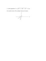
D. Vector addition. Give the expressions for the comy
........
ponents of the resultant in terms of the components
c...............................
.
.
..
of the addends. Demonstrate the equivalence of the
........... ....
.......... ........
.
.
.
.
.
.
.
graphical and analytic methods of finding a vector
.
.
b
..
....
...........
.......... a ....................
.

sum. See the diagram to the right.
.
.
.
.
.
.
.
.
......... .................................
E. Give the expression for vector subtraction in terms of
.....................................
− bx −
→ x
←−−− ax −−−→←
components. You may also wish to demonstrate the
c
−
−
−
−
−
−
−
→
←
−
−
−
−

−
−
−
x
equivalence of the graphical and analytical methods
of vector subtraction.
F. Show how to find the magnitude and angles with the coordinate axes, given the components.
Explain that calculators give only one of the two possible values for the inverse tangent
and show how to determine the correct angle for a given situation.
G. State that two vectors are equal only if their corresponding components are equal. State
that many physical laws are written in terms of vectors and that many take the form of
an equality between two vectors. Expressions for the laws are then independent of any
coordinate system.
IV. Multiplication involving vectors.
A. Multiplication by a scalar. Give examples of both positive and negative scalars multiplying
a vector. Give the components of the resulting vector as well as its magnitude and direction.
Remark that division of a vector by a scalar is equivalent to multiplication by the reciprocal
of the scalar.
B. Scalar product of two vectors (may be postponed until Chapter 7). Emphasize that the
product is a scalar. Give the expression for the product in terms of the magnitudes of the
vectors and the angle between them. To determine the angle, the vectors must be drawn
with their tails at the same point. Point out that a · b is the magnitude of a multiplied
by the component of b along an axis in the direction of a. Explain that a · b = 0 if a is
perpendicular to b.
C. Either derive or state the expression for a scalar product in terms of Cartesian components.
See the discussion leading to Eq. 3—23. Specialize the expression to show that a · a = a2 .
Show how to use the scalar product to calculate the angle between two vectors if their
components are known. Consider problem 31.
D. Vector product of two vectors (may be postponed until Chapter 12). Emphasize that the
product is a vector. Give the expression for the magnitude of the product and the right

hand rule for determining the direction. Explain that a × b = 0 if a and b are parallel.
Point out that |a × b| is the magnitude of a multiplied by the component of b along an axis
perpendicular to a and in the plane of a and b. Show that b × a = −a × b.
E. Either derive or state the expression for a vector product in terms of Cartesian components.
See the discussion leading to Eq. 3—30. Give students the useful mnemonic for the vector
ˆ written in that order clockwise around a circle.
products of the unit vectors ˆi, ˆj, and k,
One starts with the first named vector in the vector product and goes around the circle
toward the second named vector. If the direction of travel is clockwise the result, is the
third vector. If it is counterclockwise, the result is the negative of the third vector.
SUGGESTIONS
1. Assignments
a. Use questions 2, 3, and 4 to discuss properties of vectors. Questions 1 and 5 deal with
vector addition and subtraction. Question 6 deals with the signs of components.
b. Ask students to use graphical representations of vectors to think about problems such as
8 and 10.
18

Lecture Notes: Chapter 3


2.
3.

4.

5.

6.

c. Problems 3, 4, and 8 cover the fundamentals of vector components. Problems 5 and 6 stress
the physical meaning of vector components. Some good problems to test understanding of
analytic vector addition and subtraction are 13, 18, 19, and 23.
d. Unit vectors are used in problems 14, 15, 16, and 20.
Demonstrations
Vector addition: Freier and Anderson Mb2, 3.
Audio/Visual
a. Numbers, Units, Scalars, and Vectors; VHS video tape, DVD; Films for the Humanities
and Sciences (PO Box 2053, Princeton, NJ 08543—2053; www.films.com).
b. Vector Addition – Velocity of a Boat ; from AAPT collection 1 of single-concept films;
DVD; available from Ztek Co. (PO Box 11768, Lexington, KY 40577—1768, www.ztek.com)
and from the American Association of Physics Teachers (AAPT, One Physics Ellipse,
College Park, MD 20740-3845, www.aapt.org).
c. Vectors; Cinema Classics DVD 1: Mechanics (I); available from Ztek Co. and from the
AAPT (see above for addresses).
d. Vector Addition; Physics Demonstrations in Mechanics, Part III; VHS video tape, DVD;
≈3 min; Physics Curriculum & Instruction (22585 Woodhill Drive, Lakeville, MN 55044;
www.PhysicsCurriculum.com)
Computer Software
a. Vectors; Richard R. Silbar; Windows and Macintosh; available from Physics Academic
Software (Centennial Campus, 940 Main Campus Drive, Suite 210, Raleigh, NC 27606—
5212; www.aip.org/pas).
b. Vectors; Windows and Macintosh; WhistleSoft, Inc.; available from Physics Academic
Software (see above for address).
Computer Project
Have students use a commercial math program or write their own computer programs to
carry out conversions between polar and Cartesian forms of vectors, vector addition, scalar
and vector products.
Laboratory
Bernard Experiment 4: Composition and Resolution of Coplanar Concurrent Forces. Students

mathematically determine a force that balances 2 or 3 given forces, then check the calculation
using a commercial force table. They need not know the definition of a force, only that the
forces in the experiment are vectors along the strings used, with magnitudes proportional to
the weights hung on the strings. The focus is on resolving vectors into components and finding
the magnitude and direction of a vector, given its components.

Chapter 4

MOTION IN TWO AND THREE DIMENSIONS

BASIC TOPICS
I. Definitions.
A. Draw a curved particle path. Show the position vector for several times and the displacement vector for several intervals. Define average velocity over an interval. Write the
definition in both vector and component form.
B. Define velocity as dr/dt. Write the definition in both vector and component form. Point
out that the velocity vector is tangent to the path. Define speed of the magnitude of the
velocity.
C. Define acceleration as dv/dt. Write the definition in both vector and component form.
Point out that a is not zero if either the magnitude or direction of v changes with time.
Lecture Notes: Chapter 4

19