TÓM tắt LUẬN án TIẾNG ANH nghiên cứu động thái ẩm của đất trong kỹ thuật tưới nhỏ giọt để xác định chế độ tưới hợp lý cho cây nho lấy lá trên vùng khan hiếm nước

MINISTRY OF EDUCATION – MINISTRY OF AGRICULTURE
AND TRAINING
AND RURAL DEVELOPMENT
VIETNAM ACADEMY FOR WATER RESOURCES
SOUTHERN INSTITUTE OF WATER RESOURCES RESEARCH
--------------------------

TRAN THAI HUNG

RESEARCH ON SOIL MOISTURE DYNAMIC
OF DRIP IRRIGATION TECHNIQUE IN ORDER TO DETERMINE
THE SUITABLE IRRIGATION SCHEDULE FOR GRAPE LEAVES
IN THE WATER SCARCE REGION

MAJOR IN: WATER RESOURCES ENGINEERING
CODE: 9 58 02 12

SUMMARY OF ENGINEERING PHD DISSERTATION

HO CHI MINH CITY - 2018


The dissertation has been completed at:
SOUTHERN INSTITUTE OF WATER RESOURCES RESEARCH

SCIENTIFIC SUPERVISORS:
1. ASSOC PROF. DR VO KHAC TRI
2. PROF. DR LE SAM

Reviewer 1:
Reviewer 2:

Reviewer 3:

The dissertation will be defended in front of the Board of thesis
examiners – National Level
Meeting at:
SOUTHERN INSTITUTE OF WATER RESOURCES RESEARCH
658 Vo Van Kiet avenue, Ward 01, District 05, Ho Chi Minh City
At: ……...o’clock, Date …..… month ……………… year 2018

The dissertation is stored in:
- National Library of Vietnam
- Library of Vietnam Academy for Water Resources
- Library of Southern Institute of Water Resources Research


-1INTRODUCTION
1. RESEARCHING IMPERATIVE
Ninh Thuan and Binh Thuan are two provinces in the driest region of
the South Central part of Vietnam where there is the lowest precipitation of
the country and the unequal distribution by time. Therefore, water resources
for production should be utilised reasonably. The research on suitable water
saving irrigation schedule for high economic crops is very important and
necessary. Previous studies have often focused on the aspect of crops
irrigation schedule for each irrigation technique, not much attention to soil
moisture dynamic in the space of the active roots.
In the World, grape leaves (Vitis Amurensis) is cultivated a lot in USA,
Turkey, Greece, Brazil… In Vietnam, the grape leaves variety named IAC
572 has been imported from Brazil by YERGAT FOOD Co., Ltd and Binh
Thuan Socioeconomy development Centre (SEDEC) since 1999÷2010 for
cultivating and exporting leaf production. Due to Grape leaves suitable for

natural conditions in the South Central region (Ninh Thuan, Binh Thuan,
Dong Nai provinces… so the plants developed very well and obtained high
profit. There have not been any studies on suitable irrigation schedule for
Grape leaves so far, especially in the water scare tropics (droughty region)
of the South Central part. Therefore, Research on soil moisture dynamic of
drip irrigation technique in order to determine the suitable irrigation
schedule for Grape leaves in the water scarce region of the South Central
part of Vietnam was done, it aimed for clarifying the current urgent matters.
2. OBJECTIVES, OBJECT, SCOPE, CONTENTS AND METHODS
Objectives:
(1) Determine water infiltration spread and soil moisture dynamic of
drip irrigation technique;
(2) Propose the suitable schedule of water saving irrigation (drip
irrigation technique) for Grape leaves cultivated at the water scarce region
(the droughty one) in the South Central part, consisting of: Irrigation
frequency, water amount and irrigation time for each growth stage;
Research object: Research for a plant: Grape leaves in the water scarce
region of Ninh Thuan and Binh Thuan; farming technique was row (furrow).
The main irrigation was drip one (sprinkler only improved microclimate);
Research scope: at the water scarce region (the droughty one) of
Vietnam, including two provinces: Ninh Thuan and Binh Thuan; weather
condition is sunny and hot, less precipitation; main soil is fine sand; privation
of water surface condition; water saving irrigation experiment was carried
out at Binh Thuan province;
Research contents: Overview of research field;


-2Field survey, design and establishment of the experimental model for
researching on suitable irrigation schedule for Grape leaves;
Experiment of irrigation, observation of water infiltration and soil

moisture dynamic by time and space. Establishment of correlation and linear
regressions of water infiltration and soil moisture dynamic;
Experiment of plant developing and growing process following the
frequency, water amount and irrigation time for growth stages of a seasonal
crops. Establishment of correlation and linear regressions of variables
including: Meteorology (temperaturer, humidity, sunshine, wind,
precipitation, evaporation) – Crop water requirement - Crop yields;
Application of the Coup Model for simulating moisture and heat
transfer in the soil-plant-air system of drip irrigation technique;
Propose the suitable schedule of water saving irrigation (drip irrigation
technique) for Grape leaves;
Approachability: Approached comprehensively, systematically and
practically, from general to detail; Inherited, selected knowledge experience,
researches and databases; Approached ecosystem, sustainable and effective
development; Minimized waste of land and water resources;
Inherited/applied modern science and technology, achievements in irrigation
and production, harvest and advanced products preservation.
Research method: Theoretical analysis, collection and systematization;
Selective inheritance and analysis of the research experience; Field survey;
Laboratory and field experiments; Statistical data analysis; Mathematical
modeling of water infiltration and moisture dynamics in drip irrigation.
3. SIGNIFICANCES AND NEW CONTRIBUTIONS OF THE THESIS
Scientific significances:
The research has established the pF Retention curve for cultivated soil
– fine sand (named: Dystri Haplic Arenosols-ARh.d) of the water scarce
region (the droughty one) to be the scientific basis for determining the
suitable schedule of water saving irrigation for dry crops;
The research has established the correlation of Soil-Water-CropsClimate to be the scientific basis of applied researches in irrigating for dry
crops at the water scarce region (the droughty one);
The research has identified basic criteia of irrigation research and

efficiency by drip irrigation technique for Grape leaves at the water scarce
region (the droughty one) in the South Central part of Vietnam.
Practical significances:
Grape leaves are of high economic value, but water lack for irrigation is
an issue that hinders large development. Research results will help farmers


-3to save and improve the water use efficiency, serving the plant development
on a larger scale to become a strong crop;
The research results are a reasonable choice for the conversion of crop
structure towards diversification of highly economical (sustainable) crops
and adaptation to natural conditions in water scarce region;
Applying research results to simplify the irrigation work, contributing
to the plan for irrigation and development of exploitative and utilizable
models of land-water resources for sustainable production and
environmental protection.
New contributions of the thesis:
(1) Established the Soil Water Retention curves (pF) for cultivated soil
(named: Dystri Haplic Arenosols-ARh.d) in order to effectively develop drip
irrigation technique for every crops at the water scarce region (the droughty
one) in the South Central part of Vietnam;
(2) Simulated water infiltration and soil moisture dynamic in the
cultivated soil layer (active roots area) of the Grape leaves;
(3) Propose the suitable schedule of water saving irrigation (drip
irrigation technique) for Grape leaves cultivated at the water scarce region
(the drought one) in the South Central part of Vietnam.
4. THE THESIS STRUCTURE
The thesis is presented in 136 pages, consisting of 36 tables, 53
illustrative figures and explanation. The main thesis contents are 4 main
chapters, Introduction and Conclusions - Recommendations, as follows:

Introduction
Chapter 1: Overview of the research field;
Chapter 2: Theoretical basis and experimental layout;
Chapter 3: Experimental results and simulation of water infiltration,
soil moisture dynamic of drip irrigation technique;
Chapter 4: Experimental results and establishment of the suitable
irrigation schedule for Grape leaves in the water scarce region;
Conclusions and Recommendations.
The annex is presented in 145 pages, consisting of 105 tables and 99
illustrative figures and explanation "Summarizing the planting, care and
harvesting of Grape leaves".
CHAPTER I: OVERVIEW OF THE RESEARCH FIELD
I.1 RESEARCH ON WATER MOVEMENT IN SOIL-WATERPLANT SYSTEM
The water regime of the soil is considered to be consisting of the
phenomena of water entering the soil, its movement, keeping it in the soil
layers and consuming it from the soil. Scientists believe that water


-4infiltration in soil can be divided into two phases: (1) Unstable infiltration,
and (2) Permeability one. Research on water spread in the soil in order to
determine the irrigation method and suitable water amount for each plant to
improve water efficiency.
I.2 STUDY ON HYGROSCOPIC PRESSURE AND SOIL MOISTURE
TO APPLY FOR CROP IRRIGATION AND DRAINAGE
There are two methods to determine the hygroscopic pressure of the
soil: (1) Direct measurement using measuring devices (Tensiometer,
Capilarimeter or Vacum chamber); (2) Indirect method is the utilization of
instruments to measure certain parameters related to hygroscopic pressure by
dependency functions, then calculate the hygroscopic one.
Determination of soil moisture by various methods: Weight, block and

thermal capacity, Neutron tube, Time Domain Reflectrometry TDR);
A soil water retention curve (pF) of each soil type is established to
indicate the relationship between the hygroscopic pressure (h) and the soil
moisture (θ). There are three methods to establish the pF retention curve:
theory, experiment and semi-experiment. Application of the pF curve to:
forecast irrigation demand for crops; establish the relationship between
moisture-hygroscopic pressure-root density and water uptake of plant;
evaluate salt transportation and soluble spread in soil; serve the irrigation for
dry crops... Experimental research on the pF curve establishment to calculate
the available soil water and readily available soil water for plants and
determie the suitable water-saving irrigation schedule at the scarce region
(droughty one) in the South Central region is almost unnoticed. Therefore,
in order to improve the water use efficiency in production, it is necessary to
establish the pF retention curve;
Experimental study on infiltration to inspect water lack/redudant
irrigation is little interested in performing, mainly in analysis of physical and
chemical properties, although results of this infiltration study are very
important, because it is possible to happen redudant water during extended
irrigation time (water will penetrate through active root zone). Therefore,
most of the farmers have irrigated by traditional method, the irrigation time
and water amount depend on the subjective people who is directly producing,
causes a lot of waste water.
Currently, water saving irrigation technique has been applied widely in
the world, countries like USA, Israel, Australia, Spain, Germany... have
many experiences and achievements in this field, technological application
and management of water saving irrigation in agricultural production, it can
replace most conventional irrigation systems and bring high economic
efficiency. In Vietnam, farmers have step by step replaced traditional

-5irrigation methods by this irrigation system, helping to save water and
improve productivity and product quality.
Previous research has not yet paid much attention to soil moisture
dynamic in the active root zone, so it has not been applied to determine the
irrigation schedule for dry crops. Soil moisture of different irrigation
techniques is different in time and space, so when drip irrigation technique
is applied to practical production, there should be specific research on this
matter, in which soil moisture is measured by the hours of the day, to see
crops’ effective water absorption, avoiding water lack/redudant irrigation
when the optimal moisture zone exceeds or less than root space, then the
correct irrigation rate will be determined for the following seasons
Irrigation schedule studies have been performed with a number of
different methods for many dry crops. However, published results that
determine the actual daily meteorological conditions to ensure sufficient
water for crops have not been widely available yet, which limits the farmers’
irrigation work, especially at the water scarce region (droughty one) in the
South Central part.
Studies on vines in Vietnam are quite extensive, however the irrigation
study has been performed very limited for a long time, it is no longer suitable
for the present and future. Grape leaves is new, promising and economically
productive in Vietnam, its irrigation schedule has been performed, the
irrigation is subjective and mainly by the traditional method (waste water).
Therefore, the scientific basis of irrigation schedule and care for Grape
leaves is necessarily studied and determined in detail, especially in drip
irrigation at the water scarce region in the South Central part.
I.3 CHARACTERISTICS OF RESEARCH REGION
Ninh Thuan and Binh Thuan provinces have the most dry and rainy
climate of Vietnam. Although the rivers and reservoirs at two provinces are
quite plantiful, but due to the uneven rainfall in space and time, they are
severely depleted in the dry season. Annual crop losses due to drought are

high. In 2016, total area must stop producing in Ninh Thuan about 10,260ha:
Winter-Spring crop was 5,775ha (rice 2,645ha, other farm produce 3,130ha);
Summer crop was 4,495ha of rice. In Binh Thuan province, the total area of
annual crops damaged until 2nd, 2016 was 1,400ha, including 150ha of rice
(concentrated in districs as: Duc Linh 97ha, Ham Thuan Bac 19ha, Ham Tan
34ha), 300ha dragon fruit, 200ha cashew, 700ha sugarcane ... in Ham Tan.
The fallow land area of the two provinces is quite rich, but due to the
inadequate condition of the water source so local people can not cultivate
regularly and it greatly impact on the social of the whole region. Therefore,
the application of water saving irrigation solution for crops is very necessary.


-6CHAPTER II
THEORETICAL BASIS AND EXPERIMENTAL LAYOUT
II.1 THEORETICAL BASIS
II.1.1 Theoretical basis of water movement in the soil
Darcy’s Law (for water flow in the saturated soil)
Flow discharge passes the unit of area A of the saturated soil mass:
𝐻2−𝐻1
𝑄 = 𝐾 ∗ ( ∆𝐿 ) ∗ 𝐴
(2.1)
Where: H1 and H2: hydraulic head at inlet and outlet (cm);
ΔL: the length of the saturated soil mass following the flow (cm);
A: area of the saturated soil mass is perpendicular to the flow (cm2);
Q: Flow discharge passes the saturated soil mass (cm3/s);
The stable permeability passes the unit of area A in per time unit:
𝑄
𝑉 =𝐴 = 𝐾∗𝑗
(2.2)
Where: K: the hydraulic conductivity (cm/s);

𝐻2−𝐻1
J: the hydraulic gradient = ∆𝐿 (cm/cm);
The water flow in the unsaturated soil
The water flow in the unsaturated soil by Richards (1931):
𝜕𝜓
𝜕𝐶𝑣
𝑞𝑤 = −𝑘𝑤 ( 𝜕𝑧 − 1) − 𝐷𝑣 𝜕𝑧 + 𝑞𝑏𝑦𝑝𝑎𝑠𝑠
(2.3)
Where: kw: the unsaturated hydraulic conductivity;
ψ: the water tension;
z: infiltration depth;
Cv: the concentration of vapour in soil air;
Dv: the diffusion coefficient for vapour in the soil;
qbypass: bypass flow in the macro-pores;
qmat: the matrix flow;
qw: total water flow is the sum of qmat, qv (vapour flow), and qbypass;
The general equation for unsaturated water flow follows from the law
of mass conservation:
(𝜃 − 𝜃 )
(𝜃 − 𝜃 )
𝑞
𝑞 = 1 ∆𝑡 2 ∆𝑧 (2.7) or
= 2 ∆𝑡 1
(2.8)
∆𝑧
Where: θ: the soil water content;
Equations (2.3) and (2.7) are two basic ones to calculate the soil water
content.
II.1.2 Soil hydraulic functions
a) Water retention curve (pF)

Actual water tension, , by Brook & Corey (1964), is given by:
𝜓 −𝜆

𝑆𝑒 = (𝜓 )
𝑎

(2.11)

Where: ψa: the air-entry tension; λ: the pore size distribution index;


-7The effective saturation, Se, is defined as:
𝜃−𝜃
𝑆𝑒 = 𝜃 − 𝜃𝑟
𝑠

(2.12)

𝑟

Where: θ: the actual water content; θs: the porocity; θr: the residual
water content (or water content that gradient dθ/dh becomes zero);
The water retention function by Van Genuchten (1980), has been
introduced:
1
𝑆𝑒 = (1+(𝛼𝜓)g𝑛 )g𝑚
(2.13)
Where: α, gn and gm: are empirical parameters;
b) Unsaturated Conductivity
The unsaturated conductivity, kw* is given by Mualem (1976):

2

(𝑛+2+ )

𝜆
∗
𝑘𝑤
= 𝑘𝑚𝑎𝑡 𝑆𝑒
(2.16)
If function (2.11) for water retention is used, the unsaturated
conductivity, kw* is definded as:

𝜓 2+(2+𝑛)𝜆
𝜓

∗
𝑘𝑤
= 𝑘𝑚𝑎𝑡 ( 𝑎 )

(2.17)

Where: kmat: the saturated matrix conductivity;
n: a parameter accounting for pore correlation and flow path tortuosity;
Using the Van Genuchten equation (2.13), kw* is given:
−1

∗
𝑘𝑤

= 𝑘𝑚𝑎𝑡

(1−(𝛼𝜓)𝑔𝑛 (1+(𝛼𝜓)𝑔𝑛 )−𝑔𝑚 )

2

𝑔𝑚

(1+(𝛼𝜓)𝑔𝑛 ) 2

(2.18)

Where: α, gn and gm: are empirical parameters; (the same as (2.13));
As alternative options to the equations of Mualem eqs. (2.16)÷(2.18) the
unsaturated hydraulic conductivity, kw*, can either be caluclated as a simple
power function of relative saturation:
𝜃 𝑃𝑛𝑟

∗
𝑘𝑤
= 𝑘𝑚𝑎𝑡 (𝜃 )

(2.19)

𝑠

Or as a simple power function of effective saturation:
𝑃
∗
𝑘𝑤
= 𝑘𝑚𝑎𝑡 𝑆𝑒 𝑛𝑒

(2.20)
Where: Pnr, and Pne: parameters;
Se: the effective saturation;
kmat: the saturated matrix conductivity;
θs: the water content at saturation; θ: actual water content;
The total hydraulic conductivity close to saturation is calculated as:
∗
𝑘𝑤

∗ (𝜃 −𝜃 ))+
(𝑙𝑜𝑔(𝑘𝑤
𝑠
𝑚

𝑘𝑠𝑎𝑡
𝜃−𝜃𝑠 +𝜃𝑚
𝑙𝑜𝑔(
))
𝜃𝑚
𝑘𝑤(𝜃 −𝜃 )
𝑠 𝑚

= 10
(2.21)
Where: ksat: the saturated total conductivity, including the
∗ (𝜃
macropores, 𝑘𝑤
𝑠 − 𝜃𝑚 ): hydraulic conductivity below
(𝜃𝑠 − 𝜃𝑚 ) at ψmat, calculated from equations (2.16) ÷ (2.18);

-8c) Soil water availability and readily available soil water: Following
FAO, soil water availability in the layer (i) with thickness dz:
AW(i) = 1000*(θfc – θwp)* dz(i) = 1000*θaw(i) * dz(i) (mm)
(2.22)
Where: AW: available soil water in the layer i) with thickness dz (mm).
θaw, θfc: available water content and field capacity (m3/m3 or cm3/cm3);
θwp: water content at wilting point (m3/m3 or cm3/cm3);
dz(i): thickness of soil layer (i) (m).
Total available water content of all soil layers is calculated as:
𝑇𝐴𝑊 = ∑𝑛1 𝐴𝑊(𝑖) = 1000 ∑𝑛1 𝜃𝑎𝑤(𝑖) ∗ 𝑑𝑧(𝑖)
(mm) (2.23)
Where: i = 1 → n: ascending order of soil layer.
TAW: Total available water content (cumulation) of all soil layers z.
- Readily available water (RAW) is calculated as:
RAW = p * TAW
(mm) (2.24)
Where: RAW: the readily available soil water in the layer z.
p: average fraction of (TAW) that can be depleted from the root
zone before moisture stress (reduction in ET) occurs [0 ÷ 1].
II.2 CALCULATION OF WATER REQUIREMENT FOR CROPS
Total evaporation of a irrigation frequency (CK) n:
𝐸𝑝𝑎𝑛(𝑛) = ∑

𝑛

𝑖=1

𝐸𝑝𝑎𝑛(𝑖)

(mm)

(2.25)

Reference crop evapotranspiration of the irrigation frequency (ETo):
ETo(i) = Kpan * Epan(n)
(mm) (2.26)
Where: Epan(i): Total daily evaporation (mm); Kpan: pan coefficient;
n: irrigation frequency: 2 days (CK2), 3 days (CK3) or 4
days (CK4) per time;
Crop evapotranspiration or crop water need:
ETc = Kc * ETo (2.27) or Wcrop = Kc*ETo
(mm) (2.28)
Crop irrigation requirement (basic amount) of the irrigation frequency n:
Ist(n) = ETc – P(n)
(mm) (2.29)
Where: Kc: crop factor;
P(n): effective precipitation of the irrigation frequency n (mm);
Ist(n): Crop irrigation requirement of the irrigation frequency n (mm);
After calculating Ist (basic irrigation amount) of the irrigation frequency
n (mm), established more 2 other water amounts of experimental irrigation
for comparing: changed up and down 25% of Ist (called: high and low
irrigation amount), the coresponding factors: m(1) = 1.25 (high water level),
m(2) = 1.00 (basic water level or medium one), m(3) = 0.75 (low water level).
Irrigation water rate for every experimental block (j) of the irrigation
frequency n is calculated as:
Im(j) = m(j) * Ist(n)/Kef = m(j) * (ETc – P(n))/Kef
(mm) (2.30)

-9Total Irrigation water amount for every experimental block (j):
Wblock(j) = Im(j) * Fblock = Im(j) * 10-3 * (1,1 * bi * Lb)(m3) (2.31)
Where: Im(j): Irrigation water rate for every experimental block (j);
Kef: drip irrigation system efficiency; m(j): water level factor;
Wblock(j): Total water amount for every experimental block (j) (m3);
Fblock: canopy shaded area on the ground at 12:00 (m2);
10−3: factor of unit conversion from mm to m;
Bi, Lb: canopy shaded width and length on the ground at 12:00 (m).
Irrigation experiment and observation of crop data was carried out in
three seasons including: growing and developing stages; changes of treetrunk, leaves, roots and mass of living organisms...
II.3. EXPERIMENTAL LAYOUT
II.3.1. Location and characteristics of the experimental model
The experimental model was located at the South of the National
highway No 1A (between the National highway 1A and the East sea), at
Thuan Quy Commune, Ham Thuan Nam District, Binh Thuan Province;
Total area was 20,000m2 (shown in Figure 2.7). The experimental
period was in 3 crop seasons (dry ones), from January, 2012 to May, 2013.

II.3.2. Experimental research content
Description of soil profile, test of the physical and chemical properties
of soil and irrigation water; Set up the experimental model;
Experiment for establishing of the Soil Water Retention curves (pF);


- 10 Experiment for determining the saturated hydraulic conductivity at the
field and in the laboratory;
Experiment of water infiltration and establishment of correlation about
soil moisture dynamic;
Meteorological measurement for determining the irrigation schedule;
Experimental Irrigation and observation of crop development;

Result analyses and proposal of the suitable irrigation schedule for
Grape leaves at the water scarce region in the South Central part of Vietnam;
CHAPTER III:
EXPERIMENTAL RESULTS AND SIMULATION OF WATER
INFILTRATION, SOIL MOISTURE DYNAMIC OF DRIP
IRRIGATION TECHNIQUE
III.1 STEADY INFILTRATION AT THE FIELD AND IN THE
LABORATORY OF SATURATED SOIL
At the field, the layer 0÷20cm has a hydraulic conductivity of 1.176
cm/minute, layer 20÷40cm is 1.152cm/min, layer 40÷60cm is 1.111 cm/min.
In the laboratory, the hydraulic conductivity of layer 0÷20cm is high,
vertical conductivity: kz = 1.848cm/min; horizontal one: kr = 1.510 cm/min.
III.2 WATER INFILTRATION PROCESS
III.2.1 Infiltration process at the field
The statistical analysis results showed that the infiltration depth (Z) and
radius on the surface (R) at the cultivated area were larger than that one at
the non-tree place (KoTC):
CK2: Despite surface evaporation, the soil still contains high moisture,
so water infiltrated into the horizontal direction more than the deep one;
CK3: moisture content in soil was lower than CK2 so the water
infiltrated into all three directions: horizontal, oblique and vertical ones;
CK4: it had a long time of irrigation frequency so the soil was drier and
the moisture content decreased more than CK2 and CK3, the permeability
velocity in CK4 was the highest, water infiltrated into the deep direction
more than the horizontal one;
Non-tree place (KoTC): Zck2max: 43.37cm, Rck2max: 21.60cm;
Zck3max: 45.13cm, Rck3max: 20.1cm; Zck4max: 45.61cm, Rck4max: 18.38cm;
Grape leaves cultivation place with drip irrigation technique (TKN):
Zck2max: 44.53cm, Rck2max: 23.4cm; Zck3max: 46.03cm, Rck3max: 21.50cm;
Zck4max: 47.53cm, Rck4max: 19.95cm;

Graphing correlative relationship between the factors: Z, R, W, t, VZ,
VR, the determination coefficients of correlation were high (R2 > 0.90)


- 11 Z 50
(cm) 40
30
20
Z = 9.3112ln(t) - 10.912
R² = 0.9344

10
0
0

60

R 30
(cm) 25
20
15
10
5
0

120 180 240 300 360 420
t (minute)

R = 4.3998ln(t) - 0.5178
R² = 0.9818

0

60

120 180 240 300 360 420
t (minute)

Figure 3.5: Correlation graph between the factors of two-day irrigation
frequency (CK2) (At the tree place with water saving irrigation)
III.2.2 Infiltration process at the laboratory
The observation results of infiltration process at the laboratory had the
tends like the field results, as follows: Zckmax: 47.7cm, Rck4max: 25.2cm;
Graphing correlative relationship between the factors: Zlab, Rlab, W, t,
Vzlab, VRlab, the determination coefficients of correlation were high (R2 >0.90)
III.3 WATER MAINTENANCE FEATURE AND AVAILABLE WATER
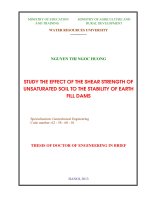
III.3.1 The pF Retention curve (pF curve)
Applied Van Genuchten’s model (1980) for establishing the pF curve to
determine soil moisture dynamic, correlation coefficient R2 from 0.96 ÷ 0.99.
The pF curve of six soil layers are typical for the fine sandy soil with
relatively uniform curves and gentle slope.
Table 3.4: Measurement results of the pF Retention curve (sample mean)
Pressure
h (pF)
Order
h (cm)
h (bar)
Layer (cm)
1
0÷10
2

10÷20
3
20÷30
4
30÷40
5
40÷50
6
50÷60
7
0÷40
8
0÷60

0.0
0.0
0.0

0.4
2.5
0.002

39.10
35.93
35.10
31.60
33.00
32.23
35.43
34.49

35.00
31.33
31.57
29.57
30.43
30.03
31.87
31.32

Soil moisture content (% volume)
1.0
1.5
1.8
2.0
2.5
4.2
10.0
31.6
63.1
100.0
316.2 15848.9
0.010
0.031
0.062
0.098
0.310
15.543
Measured sand box
Measured pF Box

33.90
23.40
13.70
12.93
11.30
5.57
29.23
21.33
12.40
12.10
11.67
3.76
29.80
21.33
11.77
11.30
10.70
3.82
28.07
20.23
11.43
11.00
10.27
4.61
28.57
20.20
11.43
10.97
10.30
3.39

27.87
19.63
10.97
10.63
10.20
3.23
30.25
21.58
12.33
11.83
10.98
4.44
29.57
21.02
11.95
11.49
10.74
4.06

Sample mean - Layer: 10-20cm
5.000

PF

PF

Sample mean - Layer: 0-10cm
5.000
4.000
3.000

2.000
1.000
.000

4.000
3.000
2.000
1.000

R² = 0.9835

R² = 0.9747

.000
0

10

20

30

40

Moisture content (%)

0

10

20
30
40
Moisture content (%)


5.000
4.000
3.000
2.000
1.000
.000

Sample mean - Layer: 20-30cm

Sample mean - Layer: 30-40cm
PF

PF

- 12 -

R² = 0.9794
0

10

20

5.000

4.000
3.000
2.000
1.000
.000

30
40
Moisture content (%)

R² = 0.9838
0

10

20

30

10

20

30
40
Moisture content (%)

Sample mean - Layer: 50-60cm
PF

PF

Sample mean - Layer: 40-50cm
5.000
4.000
3.000
2.000
1.000
.000

R² = 0.9861
0

40

5.000
4.000
3.000
2.000
1.000
.000

R² = 0.9828
0

10

20

Moisture content (%)

30
40
Moisture content (%)

Figure 3.10: The pF retention curve by soil layer
Table 3.5: Cumulative water reserves, available water
and readily available water for Grape leaves
Order

1

Layer
(cm)

θfc
(cm3/
cm3)

Wfc
(mm)

TWfc
(mm)

θ wp
(cm3/
cm3)

Wwp

(mm)

0÷10 0,1293 12,93 12,93 0,0557 5,57

TWwp
(mm)

θaw
(cm3/
cm3)

AW
(mm)

5,57 0,0736 7,36

TAW Factor RAW
P
(mm)
(mm)

7,36

TRAW
(mm
water)

θp
(cm3/
cm3)

θp
(%
TT)

0,35

2,58

2,58

0,1036 80,08

2 10÷20 0,1210 12,10 25,03 0,0376 3,76

9,33 0,0834 8,34 15,70 0,35

2,92

5,50

0,0918 75,87

3 20÷30 0,1130 11,30 36,33 0,0382 3,82

13,15 0,0748 7,48 23,19 0,35

2,62

8,12

0,0868 76,82

4 30÷40 0,1100 11,00 47,33 0,0461 4,61

17,76 0,0639 6,39 29,58

-

-

-

-

-

5 40÷50 0,1097 10,97 58,30 0,0339 3,39

21,14 0,0758 7,58 37,16

-

-

-

-

-

6 50÷60 0,1063 10,63 68,93 0,0323 3,23

24,37 0,0740 7,40 44,56

-

-

-

-

-

Where: θfc, θwp , θaw: the water content at field capacity, wilting point and available water;
Wfc, TWfc: the water amount and total cumulative water amount of soil at field capacity;
Wwp, TWwp: the water amount and total cumulative water amount of soil at wilting point;
AW, TAW: the available water and total cumulative water amount of soil;
p : the mean factor of total water amount (TAW);
RAW, TRAW: the readily available water and total readily available water for crops;
θp : the suitable minimum water content (the point P);

III.3.2 The storage capacity of available water and the readily available
water for crops
For the soil layer containing active roots of the plant from 0 ÷ 20cm (for
plants with shallow roots near the ground surface), θfc is 25.03 mm, TAW is
15.70mm (making up 62.73% θfc). In the whole layer 0 ÷ 60cm, θfc is
68.93mm, TAW is 44.56mm (making up 64.64% θfc);
Total readily available water for widespread dry crops at the water

scarce region in the South Central part, as follows: Vine: TRAW: 10.36mm
(making up 35.0% TAW). θp: 8.76% volume (V); Dragon: TRAW:


- 13 17.75mm (60.0% TAW). θp: 7.17% V; Apple: TRAW: 22.28mm (50.0%
TAW). θp: 6.93% V; Sugar cane: TRAW: 19.22mm (65.0% TRAW). θp:
6.85% V; Vegetables: TRAW: 9.27mm (40.0% TAW). θp: 8.31% V;
Union-garlic: TRAW: 4.71mm (30.0% TAW). θp: 9.6% V.
With Grape leaves, in the soil layer containing active roots of the plant
0÷20cm, TRAW is: 5.50mm (35.0% TAW), θp: 9.18÷10.36% V. When the
soil moisture decreases to the suitable minimum water content θp, plant
should be immediately irrigated water to absorb for well development.
III.4 EXPERIMENTAL RESEARCH ON SOIL MOISTURE
DYNAMIC
III.4.1 The soil moisture dynamic following the soil depth
At the end of the irrigation frequency, maximum moisture content was
CK2, the medium one was CK3, the lowest one was CK4. At the area of
KoTC: the upper layer moisture was smaller than the lower layer one. At the
area of TKN: the moisture in the soil layer containing active roots was lower
than other layers; the bottom layer was less affected by the meteorological
factors and was not absorbed by the roots, so this layer moisture was higher
than upper layers. At traditional irrigation area (CT): the lower layer
moisture was smaller than the upper layer one because the active roots were
mainly contained at below layer getting more water than the upper one.
Water saving irrigation area (CK2) - V1
0 5 10 15 20 25 30 35 Moisture
content (%)
-5

-15

-20
-25
-30

0.5 hour
6 hours
12 hours
18 hours
24 hours
30 hours
36 hours
42 hours
48 hours

-10

Depth (cm)

Depth (cm)

-10

Traditional irrigation area (CK2) - V1
0 5 10 15 20 25 30 35 Moisture
content (%)
-5

-15
-20
-25

-30

0.5 hour
6 hours
12 hours
18 hours
24 hours
30 hours
36 hours
42 hours
48 hours

Figure 3.12: Moisture content following time and soil depth at two locations –V1

III.4.2 The soil moisture dynamic following the irrigation frequency
a) At the KoTC: moisture content comparison with θp of dry crops at
the end of the irrigation frequency, the results weree as follows: garlic
onions, vegetables, tomatoes, apples, dragon, sugarcane... When farmers
apply water saving irrigation technique, irrigation frequency should not be
longthened more than 4 days; with drought plants (sugarcane, dragon...) can
be irrigated with medium frequency (3 days), because plants with high
sensitivity to water such as vegetables, tomatoes and onions will be waterless
on the last days of the frequency. To avoid loss of productivity and product
quality after harvesting, the irrigation frequency should be short (2 days).


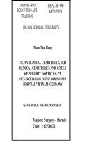
- 14 b) At the TKN: Most of soil moisture at the end of CK3 and CK4 were
less than θp, in which the moisture in layer 10 ÷ 20cm of CK4 was sometimes
equal to or approximately the moisture θwp, it made difficulty for plant water
absorption. Moisture at the end of CK2 was higher than θp, which ensures

for the crops sufficiently absorbed water to grow well.
0.0

2.5

5.0

7.5

10.0

12.5

15.0

17.5

20.0

Depth (cm)

-5

Moisture content (%)
θwp

-10

θp - Grape leaves

-15

θend of CK2 (TKN2-V1)

-20

θend of CK3 (TKN3-V1)

-25

θend of CK4 (TKN4-V1)

-30

Figure 3.15: Moisture content comparison with θwp và θp at the end of
frequencies – At the water saving irrigation area (TKN) - V1 season.
c) At the traditional irrigation area for Grape leaves (CT):
The moisture content at the end of CK3 and CK4 were lower than θp,
even CK4 was approximately θwp, when crops had high water demand, trees
absorbed water difficultly and light wilt, it was affecting the productivity and
product quality of the whole season. Moisture of CK2 was higher than θp.
0.0

Depth (cm)

-5
-10
-15
-20
-25

-30

2.5

5.0

7.5

10.0

12.5

15.0

17.5

20.0

Moisture content (%)
θwp
θp - Grape leaves
θend of CK2 (CT2-V1)
θend of CK3 (CT3-V1)
θend of CK4 (CT4-V1)

Hình 3.16: Moisture content comparison with θwp và θp at the end of
frequencies – At the traditional irrigation area (CT) - V1 season
III.5.3 The soil moisture dynamic following time (o’clock)
a) At the KoTC: the smallest moisture decrease was from
21:00PM÷3:00AM; the third one was from 3:00AM÷9:00AM; the second

one was from 15:00PM÷21:00PM and only lower than decrease from
9:00AM÷15:00PM; the largest one was from 9:00AM÷15:00PM. Layer
0÷5cm had the largest decrease, the next ones were layers 5÷10cm,
10÷15cm, 15÷20cm, 20÷25cm and 25÷30cm in turn.
b) At the TKN: Considering the moisture decrease between the soil
layers, there was a clear difference in order compared to the KoTC, due to
the roots’ water absorption moving to the trunk and leaves for
photosynthesis, metabolism for developing and thermal balance. Reduction
order was: the layer 10÷15cm had the largest decrease, the next ones were
layers 5÷10cm, 15÷20cm, 0÷5cm, 20÷25cm and 25÷ 30cm in turn.


- 15 -

Moisture content
(%)

c) At the CT: Daily moisture decrease was also as the TKN. Considering
the moisture decrease between the soil layers, there was a clear difference in
the order compared to the KoTC and TKN, the soil layer 20÷30cm had the
greatest moisture decrease, the next ones were layers 15÷20cm, 10÷15cm,
5÷10cm and 0÷5cm in turn.
5.00
4.00
3.00
2.00
1.00
0.00

15:00 21:00 3:00

9:00 15:00 21:00 3:00
9:00 Chu kỳ 21:00 3:00
9:00 15:00 21:00 3:00
9:00 15:00
(after 6 (after 12 (after 18 (after 24 (after 30 (after 36 (after 42 (after 48 mới (after 6 (after 12 (after 18 (after 24 (after 30 (after 36 (after 42 (after 48
hours) hours) hours) hours) hours) hours) hours) hours)
hours) hours) hours) hours) hours) hours) hours) hours)

-5 cm

-10cm

Time (hour)
-15 cm
-20 cm

-25 cm

-30 cm

Figure 3.18: Daily moisture decrease of soil layers - at the KoTC, CK2-V1
Moisture content
(%)

5.00
4.00
3.00
2.00
1.00
0.00

15:00 21:00 3:00
9:00 15:00 21:00 3:00
9:00 Chu kỳ 21:00 3:00
9:00 15:00 21:00 3:00
9:00 15:00
(after 6 (after 12 (after 18 (after 24 (after 30 (after 36 (after 42 (after 48 mới (after 6 (after 12 (after 18 (after 24 (after 30 (after 36 (after 42 (after 48
hours) hours) hours) hours) hours) hours) hours) hours)
hours) hours) hours) hours) hours) hours) hours) hours)

-5 cm

-10cm

Time (hour)
-15 cm
-20 cm

-25 cm

-30 cm

Moisture content
(%)

Figure 3.19: Daily moisture decrease of soil layers - at the TKN, CK2 - V1
5.00
4.00
3.00
2.00

1.00
0.00

15:00 21:00 3:00
9:00 15:00 21:00 3:00
9:00 Chu kỳ 21:00 3:00
9:00 15:00 21:00 3:00
9:00 15:00
(after 6 (after 12 (after 18(after 24 (after 30(after 36 (after 42 (after 48 mới (after 6 (after 12(after 18 (after 24 (after 30 (after 36 (after 42 (after 48
hours) hours) hours) hours) hours) hours) hours) hours)
hours) hours) hours) hours) hours) hours) hours) hours)

-5 cm

-10cm

Time (hour)
-15 cm
-20 cm

-25 cm

-30 cm

Figure 3.20: Daily moisture decrease of soil layers - at the CT, CK2 - V1

III.5 APPLIED THE COUP MODEL FOR SIMULATING SOIL
MOISTURE DYNAMIC IN THE SOIL-PLANT-AIR SYSTEM
III.5.1 Introduction of the Coup Model
The original name of the Coup Model was the Soil Model developed for

simulating the water and heat movement for any cover-crop soil by the soil
profile depth. The basic theory consists of: (1) Laws of mass and energy
conservation; (2) Flow in the soil (Darcy's Law) or temperature (Fourier's
Law).
III.6.2 Applied the Coup Model for simulating soil moisture dynamic in
the soil-plant-air system
a) Data input: Input meteorological data, irrigation water, crops (leaf,
root…), soil characteristic… to sheets as: Document, Run Info, Switches,
Parameters, Parameter tables, Model files…;
Simulation for 3 seasons: V1 from 01/01 ÷ 30/4/2012, V2 from 01/9 ÷
30/12/2012; V3 from 01/01 ÷ 30/4/2013.


- 16 b) Analysis of simulation results
Established the pF retention curve by the Coup Model based on soil
properties, these results were quite similar with the measurement results of
suction pressure in the laboratory.
Soil moisture dynamic: moisture at the beginning of the crop season was
low. After irrigating, the moisture increased and maintained higher than at
the begining time, this result was also consistent with the field actual
observation. The evapotranspiration (soil and leaf) during the irrigation and
the crop development, the amplitude was from 0.5÷4mm/day. Water
absorption of the roots was from 0÷2mm/day the evapotranspiration. The soil
temperature change was following the depth, the layer 0÷5cm was from
18÷220C, the amplitude of lower layers decreased from 1.5÷20C and quite
evenly by time. The concentrated development of active roots by simulation
result was similar to the active root development in the field.
III.6 EXPERIMENTAL DATA TEST, CORRELATION ANALYSIS
AND LINEAR REGRESSION ESTABLISHMENT
Data processing by statistical analysis, Cronbach's Alpha reliability

testing and Exploratory factor analysis. Mean different test of statistical
significance by One-way Analysis of Variance (ANOVA), in which the
Levene Statistic test - homogeneous variance, F test - statistically significant
difference (ANOVA) and Welch test - a supposition breach of heterogeneity
variances. The test results are statistically required for calculation, analyzing
and establishing linear regression equations between the factors.
Test results of correlation coefficient ensure the correlation of factors
are very closely. The regression equations are as follows:
Table 3.15: Regression equations of the water infiltration in soil
Area

Relation of
factors
f (Z) = f (t)
f (Z) = f (W, R)
f (Vz) = f (W, R)
TKN
f (R) = f (t)
f (R) = f (W)
f (VR) = f (W, R)

CK2

CK3

Z2 = 0,957t2
Z2 = 0,481W2 + 0,555R2
Vz2 =0,397W2 - 1,300R2
R2 = 0,858t2
R2 = 0,858W2

VR2 =0,554W2 - 1,417R2

Z3 = 0,969t3
Z3 = 0,596W3 + 0,445R3
Vz3 = 0,357W3 - 1,253R3
R3 = 0,838t3
R3 = 0,838W3
VR3 =0,488W3 - 1,355R3

CK4
Z4 = 0,961t4
Z4 = 0,582W4 + 0,467R4
Vz4 =0,289W4 - 1,199R4
R4 = 0,813t4
R4 = 0,813W4
VR4 = 0,432W4 - 1,296R4

Table 3.16: Test results and establishment of regression equations between
the pF retention curve – TAW(pF2) and the pF retention curve – TRAW(pF)
EigenRegression
value
equations
> 0,5 > 0,5 <0,05 <0,05 < 10 > 1
1 f(TAW) = f(θpF2) 0,946 0,868 0,004 0,004 1,00 1,998 TAW = 0,946* θpF2
2 f(TRAW) = f(θpF) 0,946 0,868 0,004 0,004 1,00 1,998 TRAW = 0,946* θpF

OrRelation of factors
der

|𝑟|

R2

F

t

VIF


- 17 Table 3.17: Regression equations of soil moisture (θzi) and the pF curve
Or- Season Area
der

1

V1
and
V3

TKN

2

V2

TKN

Layer Zi
(cm)

0÷5
5 ÷ 10
10 ÷ 15
15 ÷ 20
20 ÷ 25
25 ÷ 30
0÷5
5 ÷ 10
10 ÷ 15
15 ÷ 20
20 ÷ 25
25 ÷ 30

CK2

CK3

CK4

θz5 = 0,952*θpF
θz10 = 0,953*θpF
θz15 = 0,955*θpF
θz20 = 0,955*θpF
θz25 = 0,949*θpF
θz30 = 0,947*θpF
θz5 = 0,948*θpF
θz10 = 0,951*θpF
θz15 = 0,954*θpF
θz20 = 0,954*θpF
θz25 = 0,941*θpF

θz30 = 0,939*θpF

θz5 = 0,946*θpF
θz10 = 0,949*θpF
θz15 = 0,952*θpF
θz20 = 0,951*θpF
θz25 = 0,942*θpF
θz30 = 0,939*θpF
θz5 = 0,948*θpF
θz10 = 0,950*θpF
θz15 = 0,952*θpF
θz20 = 0,953*θpF
θz25 = 0,941*θpF
θz30 = 0,937*θpF

θz5 = 0,942*θpF
θz10 = 0,946*θpF
θz15 = 0,950*θpF
θz20 = 0,948*θpF
θz25 = 0,939*θpF
θz30 = 0,937*θpF
θz5 = 0,941*θpF
θz10 = 0,946*θpF
θz15 = 0,950*θpF
θz20 = 0,947*θpF
θz25 = 0,937*θpF
θz30 = 0,934*θpF

CHAPTER IV:
EXPERIMENTAL RESULTS AND ESTABLISHMENT OF THE

SUITABLE IRRIGATION SCHEDULE FOR GRAPE LEAVES IN
THE WATER SCARCE REGION
IV.1 IRRGATION WATER AMOUNT FOR CROPS
IV.1.1 Comparison of water amount for each irrigation time
Statistical analysis results of infiltration experiment showed that
irrigation water amounts of CK2: 1.05 liter/dripper (or 5.383m3/ha,
infiltration depth Z = 24.1cm, active root depth 14.6 ÷ 15.4cm; CK3: 1.053
lit/drip (or 5.973m3/ha, Z = 23.8cm, root depth 16.8 ÷17.7cm) and CK4:
0.8825 lit/drip (or 4.523m3/ha, Z = 23.8cm, root depth 19.0÷20.2cm) for
comparison as:
Irrigation times of A3 and A'3 (low water level m(3) in CK2) with water
content was smaller than 5.383m3/ha occupying the highest rate, it means
that the excess water was the lowest. At the end of the irrigation frequency,
the soil still maintained moisture for plants to absorb and grow well, get high
yield. At other blocks of CK2 (irrigation level m(1) and m(2)), especially CK3
and CK4 (for all m(1), m(2) and m(3)), there was a water part infiltrated deeply
and over-root zone causing water waste, at the end of CK3 and CK4,
moisture still reduced, not enough water for plants to absorb and develop.
IV.1.2 Comparison of water amount following the irrigation frequency
In 3 seasons as: (1) CK2 (comparison with Act): A1-A’1 saved 67,603
÷ 106,459m3/ha; A2-A’2 saved 162,619 ÷ 192,619m3/ha; A3-A’3 saved
227,764 ÷ 287,635m3/ha. (2) CK3 (comparison with Bct): B1-B’1 saved
74,118 ÷ 116,009m3/ha; B2-B’2 saved 150,086 ÷ 208,410m3/ha; B3-B’3
saved 226,054 ÷ 306,581m3/ha. (3) CK4 (comparison with Cct): C1 - C’1


- 18 -

Irr water amount
(m3/ha)

saved 136,881 ÷ 207,816 m3/ha; C2 - C’2 saved 215,397 ÷ 295,747m3/ha;
C3 - C’3 saved 293,913 ÷ 391,083 m3/ha.
IV.1.3 Comparison of the highest water amount - Block Cct
All experimental blocks have lower irrigation water amount than block
Cct, in which blocks with low water level (m(3)) were equal 40÷50% of Cct.
800
600
400
200
0
A1 A'1 A2 A'2 A3 A'3 Act B1 B'1 B2 B'2 B3 B'3 Bct C1 C'1 C2 C'2 C3 C'3 Cct
Block
V1: January - April, 2012
V2: September - December, 2012
V3: January - April, 2013

Leaves' development process, main branch, Block A1 (extra sprinkler irr), CK2, V1
20.0
15.0
10.0

30/04/2012

20/4/2012

25/04/2012

15/4/2012

10/4/2012

05/4/2012

30/03/2012

20/3/2012

Observation tine

25/03/2012

15/3/2012

10/3/2012

05/3/2012

29/02/2012

25/02/2012

20/02/2012

15/02/2012

10/02/2012

05/02/2012

30/01/2012

25/01/2012

20/01/2012

0.0

15/01/2012

5.0
10/01/2012

Leaf width (cm)

Figure 4.4: Total irrigation water amount for crops in three seasons
IV.2 EFFICENCY OF WATER SAVING IRRIGATION TECHNIQUE
TO CROPS’ DEVELOPMENT AND YIELD
IV.2.1 Descriptive statistics analysis of the leaf development
The statistical analysis results of harvested leaves were quite small
standard deviations compared to sample mean. Leaves of blocks with extra
sprinkler irrigation developed faster and more equally than blocks’ purely
drip irrigation. The leaves of CK2 growed faster and more equally than CK3
and CK4. In CK3 and CK4, the leaf development of blocks’ high water level
was faster than medium and less water level. Block C'3 (CK4) had some
leaves waiting for 40 days to achieve the required size. The leaf development
order is as follows: Blocks A1, A2, A3 > A’1, A’2, A’3 and Act > B1, B2,
B3 > B’1, B’2, B’3 and Bct > C1, C2, C3 > C’1, C’2, C’3 and Cct.
Leaf 1
Leaf 2

Leaf 3
Leaf 4
Leaf 5
Leaf 6
Leaf 7
Leaf 8
Leaf 9
Leaf 10
Leaf 11
Leaf 12
Leaf 13
Leaf 14
Leaf 15
Leaf 16
Leaf 17

Figure 4.5: Grape leaves’ development process in the season V1
IV.2.2 Development of the tree-trunk and active roots
The trunk perimeter of CK2 was larger than CK3 & CK4, but the
difference was a little. The roots of water-saving irrigated plants tended to
thrive in arable layer (0÷20cm) which regularly maintains moisture.


- 19 IV.2.3 Biomass of leaves and tree-trunk
The water rate of the leaves and trunk was quite large, season V2 has
more water rate than in V1 and V3; in CK2 was larger than in CK3 and CK4.
IV.2.4 Product harvest process and crop yield
Compared to the same irrigation frequencies, the leaf weight of the
sprinkler irrigation blocks was greater than in other ones. The productivity
of CK2 was higher than CK3 and CK4 (the same irrigation level). The CK2

had yield at the harvest beginning not much difference with the next harvests,
harvest time of large scale was more early than CK3 and CK4. In CK3 and
CK4, yield at the harvest beginning was low, usually concentrated in the
middle and late seasons (because the leaves growed more slowly than CK2).
The productivity order of blocks is as follows: A1, A2, A3, A’1, A’2, A’3,
Yield (ton/ha)

Act > B1, B2, B3, B’1, B’2, B’3, Bct > C1, C2, C3, C’1, C’2, C’3, Cct
10.000
8.000
6.000
4.000
2.000
0.000
A1 A'1 A2 A'2 A3 A'3 Act B1 B'1 B2 B'2 B3 B'3 Bct C1 C'1 C2 C'2 C3 C'3 Cct
Block
V1: January - April, 2012
V2: September - December, 2012
V3: January - April, 2013

WUE
(Ton/ha.m3.10^-3)

30.0
25.0
20.0
15.0
10.0
5.0
0.0

Irr productivity
(%)

Figure 4.8: Crop yield of experimental blocks - in three seasons
IV.3 WATER USE EFFICIENCY - WUE
Sprinkler irrigation blocks’ WUE were higher than purely drip and
traditional irrigation ones. Blocks’ WUE in CK2 were higher than CK3 and
CK4. In the same irrigation frequencies, WUE of low irrigation level blocks
(m(3)) was the highest, the next by medium one (m(2)) and high one (m(1)).

75.0
60.0
45.0
30.0
15.0
0.0

A1 A'1 A2 A'2 A3 A'3 Act B1 B'1 B2 B'2 B3 B'3 Bct C1 C'1 C2 C'2 C3 C'3 Cct
Block
V1: January - April, 2012
V2: September - December, 2012
V3: January - April, 2013

Figure 4.9: Water use efficiency of the whole season
V1: January April, 2012

A1
A'1
A2

A'2
A3
A'3
Act
B1
B'1
B2
B'2
B3
B'3
Bct
C1
C'1
C2
C'2
C3
C'3
Cct

V2: September December, 2012
Block

V3: January April, 2013

Figure 4.11: Irrigation productivity of the whole season


- 20 IV.4 EXPERIMENTAL DATA TEST, CORRELATION ANALYSIS
AND LINEAR REGRESSION ESTABLISHMENT
Reliable tests of irrigation and crop development data (Cronbach's

Alpha, EFA, One-Way ANOVA…) are statistically required for detailed
assessing and analyzing.
The correlation analysis results of Pearson (r > 0,5), R2 > 0,5, test of F,
t with Sig.= 0,0001 < 0,05 (reliability is 95%), VIF < 10, Eigenvalue > 1,
which are satisfied for establishing linear regression equations, as followed:
(1) f (ETo) = f (t, h, s, w, p) - (Meteorological regression)
Where: Eto: Evaporation is dependent variable; t: temperature, h: air
humidity, s: sunshine, w:wind and p: precipitation are independent variables
(2) f (Im) = f (ETo) - (Regression of irrigation water - Evaporation)
(3) f (Ym) = f (Ym) - (Regression of crop yield - irrigation water)

1

2

3

Irr. frequency

Table 4.8: Linear regression equations of factors
Order

Season
Linear
regression
equations

m1 = 1.25
2 m2 = 1.00
m3 = 0.75

m1 = 1.25
3 m2 = 1.00
m3 = 0.75
m1 = 1.25
4 m2 = 1.00
m3 = 0.75

V1 (from January 1st ÷ April 30th)
f (ETo) = f (t, h, s, w, p)
ETo(V1) = 0.112t - 0.415h + 0.308s +
0.587w - 0.049p
f (Im) = f (ETo)
f (Ym) = f (Im)
I1.25 = 0.875*ETo1.25 Y1.25 = 0.994* I1.25
I1.00 = 0.877*ETo1.00 Y1.00 = 0.994* I1.00
I0.75 = 0.879*ETo0.75 Y0.75 = 0.994* I0.75
I1.25 = 0.855*ETo1.25 Y1.25 = 0.993* I1.25
I1.00 = 0.855*ETo1.00 Y1.00 = 0.993* I1.00
I0.75 = 0.854*ETo0.75 Y0.75 = 0.993* I0.75
I1.25 = 0.858*ETo1.25 Y1.25 = 0.981* I1.25
I1.00 = 0.863*ETo1.00 Y1.00 = 0.980* I1.00
I0.75 = 0.862*ETo0.75 Y0.75 = 0.979* I0.75

V2 (from September 1st ÷ December 30th)
f (ETo) = f (t, h, s, w, p)
ETo(V2) = - 0.021t - 0.458h + 0.355s +
0.540w - 0.053p
f (Ym) = f (Im)
f (Im) = f (ETo)
I1.25 = 0.952*ETo1.25 Y1.25 = 0.997* I1.25

I1.00 = 0.951*ETo1.00 Y1.00 = 0.997* I1.00
I0.75 = 0.951*ETo0.75 Y0.75 = 0.997* I0.75
I1.25 = 0.943*ETo1.25 Y1.25 = 0.995* I1.25
I1.00 = 0.945*ETo1.00 Y1.00 = 0.996* I1.00
I0.75 = 0.945*ETo0.75 Y0.75 = 0.996* I0.75
I1.25 = 0.921*ETo1.25 Y1.25 = 0.997* I1.25
I1.00 = 0.919*ETo1.00 Y1.00 = 0.997* I1.00
I0.75 = 0.920*ETo0.75 Y0.75 = 0.998* I0.75

IV.5 THE DRIP IRRIGATION SCHEDULE FOR GRAPE LEAVES
(1) Total time of canopy development and leaf harvest is about 4 months
(2) Irrigation frequency is 2days; Apply drip irrigation level with less
water (m = 0.75);
(3) Drip irrigation amount (Im) is calculated from evaporation (ETo),
daily effective precipitation (P) and crop coefficient (Kc) following
each growing and developing stage of crops, or
(4) Drip irrigation one (Im) is also calculated with 0.725 (litter/one
tree per time) equally 3.745 (m3/one hectare per time) in order to
maintain moisture in the active root layer, avoid deep infiltration
causing waste water.


- 21 Table 4.9: Crop coefficient Kc of drip irrigation for Grape leaves
The 1st
time cut
Growing Developing
Developing tree
the top
Directs up the Directs
stage

sprout
directs down
of the
top of the trellis down
trellis
Time
10-20/01 21-31/01 01-10/02 11-20/02 21-29/02 01-10/3 11-20/3
Developing tree

0,30

0,45

0,55

0,60

0,65

0,65

0,70

0,70

0,65

0,65

0,55

8.929

12.137

14.712

14.712

13.241

14.712

14.712

16.183

14.712

14.712

12.505

11.365

15.450

18.727

18.727

16.854

18.727

18.727

20.599

18.727

18.727

15.918

10-20/9
0,25

ETo(V1) = 0,112t - 0,415h + 0,308s + 0,587w - 0,049p
I0,75 = 0,879*ETo0,75
Y0,75 = 0,994* I0,75
21-30/9 01-10/10 11-20/10 21-31/10 01-10/11 11-20/11 21-30/11 01-10/12 11-20/12 21-30/12
0,30
0,45
0,55
0,60
0,60
0,65
0,65
0,60

0,60
0,55

8.929

12.137

14.712

14.712

13.241

14.712

14.712

14.712

14.712

14.712

12.505

11.365

15.450

18.727

18.727

16.854

18.727

18.727

18.727

18.727

18.727

15.918

ETo(V1) = 0,112t - 0,415h + 0,308s + 0,587w - 0,049p
I0,75 = 0,879*ETo0,75
Y0,75 = 0,994* I0,75
Crop coefficient curve Kc
(Period from September to December)

0.80

0.80

Time

21-30/12

11-20/12

01-10/12

21-30/11

11-20/11

01-10/11

21-31/10

21-30/4

11-20/4

01-10/4

21-31/3

11-20/3

01-10/3

21-29/02

11-20/02

01-10/02

0.00
21-31/01

0.20

0.00
10-20/01

0.40

0.20

11-20/10

0.60

0.40

21-30/9

0.60

01-10/10

Kc

Kc

Crop coefficient curve Kc

(Period from January to April)

10-20/9

Kc
Irrigation
water rate
(mm)
Irrigation
water rate
(m3/ha)
Linear
regression
equations
Time
Kc
Irrigation
water rate
(mm)
Irrigation
water rate
(m3/ha)
Linear
regression
equations

The 2nd
time cut
Developing tree
the top

directs down
of the
trellis
21-31/3 01-10/4 11-20/4 21-30/4

Time

Figure 4.13: Crop coefficient curve Kc of drip irrigation for Grape leaves
CONCLUSIONS AND RECOMMENDATIONS
1. CONCLUSIONS
The thesis has achieved new major results as follows :
 As regards water spread in soil of drip irrigation technique (water
infiltration)
1.1) Investigated water infiltration spread in soil at 3 places: soil without
cultivating, plants with water saving irrigation and in the laboratory,
results as: vertical velocity (Vz) and infiltration depth (Z) are bigger than
horizontal velocity (VR) and average radius of wetting front on horizontal
direction (R). The results were showed that after irrigating in 40 ÷ 50
minutes, water spread completely covering the active root area (0 ÷


- 22 20cm deep). The establishment of correlation and linear regressions of
following variables: Z, R, W, Vz, VR, with satisfatory test results and high
correlation coefficient, linear regression models were suitable and
significant to infer the general in order to apply into production reality.
 As regards establishment of the pF Retention curve (pF curve)
1.2) Established the pF curve for cultivated soil of the water scarce region in
the South Central part, in order to apply it in calculating the readily
available soil water (RAW), the correlation is very close (R2 > 0.9).
(1.2.1) Total available soil water (TAW) in comparision with water content

is from 56.91% (layer 0÷10cm) to 64.64% (layer 50÷60cm);
(1.2.2) Total readily available soil water (TRAW) and the suitable minimum
water content (θp) for popular dry crops at the water scarce region as
follows: Vine: 10.35mm. θp: 8.76%TT; Dragon tree: 17.75mm. θp:
7.17%TT; Apple: 22.28mm. θp: 6.93%TT; Sugar-cane: 19.22mm. θp:
6.85%TT; Vegetables: 9.27mm. θp: 8.31%TT; Onion-Garlic: 4.71mm.
θp: 9.6%TT. Cultivated soil needs be irrigated to maitain moisture
content from the suitable min water content (θp) to field capacity (θfc).
 As regards research on soil moisture dynamic
1.3) Determined soil moisture dynamic at non-plant and plant places of the
water scarce region in the South Central part. The results are showed:
(1.3.1) At the KoTC: moisture increased in soil layers depth (Z), the layer
(0÷5cm) had the smallest value, the layer (25÷30cm) had the biggest one;
(1.3.2) At the TKN: moisture in the layer (0÷10cm) decreased fast because
roots absorbed water for plant development. Moisture in layer (20÷30cm)
decreased the most slowly in comparision with above layers because of
non-root, water mainly infiltrated deeply but not absorbent by roots.
Thus, from the layer (20 ÷ 30cm) to the bottom, irrigation water was less
effective for Grape leaves, so it should be paid attention to limit the
water to infiltrate deeply into this soil layer;
(1.3.3) Moisture at the TKN: CK2: moisture at the end of frequency was
higher than θp, crops were not deprived of water. CK3 and CK4: were
supplied more water than CK2, therefore a lot of water infiltrated deeply,
at the beginning and middle of the frequency, crops got enough water;
but at the end of frequency, moisture decreased and was lower than θp,
it sometimes closed to wilting point (θwp), crops were short of water. For
this reason, the CK2 for Grave leaves is suggested to develop well;
(1.3.4) At the CT: moisture decreased in the soil layer depth (Z) (because
active roots were deep). Decreasing amount of this place was greater
than the KoTC and TKN (because water mainly infiltrated deeply);

- 23 (1.3.5) In daytime moisture decreased greater than in the evening and at
night; moisture in the afternoon decreased greater than in the morning.
The greatest decreasing amount was from 9:0AM to 15:0PM. Therefore,
farmers should irrigate in the morning for crops to absorb much water
during the process of photosynthesis, metabolism and body heat balance;
(1.3.6) Established the correlation and linear regressions of variables: (a)
Infiltration, (b) pF curve and water amount in soil, (c) pF curve and water
content of each layer. Test results were satisfied and correlation
coefficient was high, linear regression models were suitable and
significant to infer the general.
 As regards research on simulation of soil moisture dynamic
1.4) Applied the Coup Model for simulating moisture and heat transfer in the
soil-plant-air system with the results approached field observations.
 Proposed the suitable schedule of water saving irrigation (drip
irrigation technique) for Grape leaves
1.5) The thesis has showed as follows:
(1.5.1) CK2 with less water level (m(3)) had the lowest excess water, the soil
ensured the moisture absorption and well development of crops to
achieve high productivity. Experimental blocks of: CK2 with m(1) and
m(2)), CK3 and CK4 supplied water infiltrated over active root area to
become waste; at the end of the irrigation frequency, moisture reduced
and crops could not absorb enough water for developing well;
(1.5.2) Less water level (m(3)) saved a lot of water in comparision with two
others irrigation levels (m(1)) and (m(2));
(1.5.3) The blocks with drip and extra sprinkler system had higher water use
efficiency than the pure drip irrigation blocks and control ones. The
blocks of CK2 had higher water use efficiency than CK3 and CK4. The
water use efficiency of blocks with less water level (m(3)) was the highest;

(1.5.4) Irrigation productivity which applied saving irrigation technique
showed that: The order of productivity in each irrigation frequency also
decreased from the low water level (m(3)) to the high water one (m(1));
(1.5.5) The trees’ development in the drip and extra sprinkler blocks was
faster and better, early and more productive harvest, concentrating and
homogenizing than the pure drip irrigation blocks and control ones;
(1.5.6) Profit of the drip and extra sprinkler blocks was higher than the pure
drip irrigation blocks and control ones. Blocks of CK2> CK3 >CK4;
(1.5.7) Established the correlation and linear regressions of variables:
Meteorology – Crop water requirement - Crop yields from the field
experiments with satisfatory test results, high correlation coefficient,
linear regression models is suitable and significant to infer the general;