Studies in Avian Biology 11

BIRD
SEA

COMMUNITIES
AT
OFF CALIFORNIA:
1975 to 1983

KENNETH
DAVID

T. BRIGGS,

B. LEWIS

WM. BRECK

and DAVID

TYLER,

R. CARLSON

Institute of Marine Sciences, University of California
Santa Cruz, California 95064

Studies in Avian Biology No. 11
A PUJ3LICATION OF THE COOPER ORNlTHOLOGICAL

Cover Photograph:

SOCJJ3l-Y

Adult (foreground) and first-winter Common Murres (Urio aolge] on Monterey Bay, California,
September 1982. Photo by W. B. Tyler.

i


STUDIES

IN AVIAN

BIOLOGY

Edited by
FRANK

A. PITELKA
at the

Museum of Vertebrate Zoology
University of California
Berkeley, CA 94720
EDITORIAL

ADVISORS

FOR SAB 11
George L. Hunt, Jr.

Joseph R. Jehl, Jr.

David G. Ainley
Daniel W. Anderson

Studiesin Avian Biology is a series of works too long for The Condor, published
at irregular intervals by the Cooper Ornithological Society. Manuscripts for consideration should be submitted to the current editor, Joseph R. Jehl, Jr., Sea
World Research Institute, 1700 South Shores Road, San Diego, CA 92109. Style
and format should follow those of previous issues.
Price: $7.00 including postage and handling. All orders cash in advance; make
checks payable to Cooper Ornithological Society. Send orders to James R. Northem, Assistant Treasurer, Cooper Ornithological Society, Department of Biology,
University of California, Los Angeles, CA 90024.
ISBN: O-935868-36-4
Library of Congress Catalog Card Number 87-073438
Printed at Allen Press, Inc., Lawrence, Kansas 66044
Issued 28 December 1987
Copyright by Cooper Ornithological

ii

Society, 1987


CONTENTS
Abstract ...........................................................
Introduction .......................................................
Methods.. .........................................................
Sampling Plan and Coverage at Sea ................................
Observation Protocols ............................................
Shoreline Methods and Coverage ...................................

Environmental Data ..............................................
Analyses ........................................................
Oceanography of the Study Area .....................................
Bathymetry ......................................................
General Characteristics of Surface Waters ...........................
Upwelling .......................................................
Important Mesoscale Features .....................................
Results ............................................................
Seabird Numbers and Status: Species Accounts ......................
Seabird Density and Biomass ......................................
Diversity and Species Composition .................................
Associations Between Species ......................................
Spatial Scales of Aggregation ......................................
Seabird Habitats .................................................
Scales of Variation in Surface Temperature ..........................
Discussion .........................................................
Variation in Biomass and Abundance ..............................
............................
Community Composition and Diversity
..............................................
Species Associations
Seabird Habitats and Habitat Choice ...............................
Acknowledgments ..................................................
.....................................................
LiteratureCited

...

111

1
3
4
4
5
5
6
7
8
8
8
9
11
11
11
47
49
52
56
58
63
64
64
66
67
68
71
71

GLOSSARY
AFN/AB:

AND ACRONYMS

Audubon Field Notes/American Birds.

NOAA: The U.S. National Oceanographic and
Atmospheric Administration; within NOAA, the
Satellite Field Service Offices of the National
Weather Service provide operational monitoring
of ocean thermal conditions. NOAA also maintains a network of oceanographic data buoys that
provided the basis for calibration of radiometric
temperature data taken from airplanes in this
study.

CalCOFI: California Cooperative Oceanic Fisheries Investigations; an agency drawing personnel, direction and support from the National Marine Fisheries Service, the California Department
of Fish and Game and the University of California. CalCOFI investigators have gathered
much of the basic information available about
fisheries, oceanography and biology of the California Current System.

North Pacific Central Gyre: The vast mass of
subtropical to temperate water occupying the
central portion of the North Pacific Ocean. The
Gyre is bounded by the California Current in the
east, North Equatorial Current in the south, Kuroshio Current in the west and the North Pacific
West Wind Drift in the north. Compared to the
California Current, surface waters of the Gyre
are relatively warm, clear, salty and well stratified in the vertical dimension.

CUZ: Coastal Upwelling Zone; the area under
direct influence of coastal upwellings (not including areas influenced only by upwelled waters
advected by offshelf eddies). On theoretical
grounds the upwelling zone is limited to about
25 to 40 km from the coast.
Cyclonic (Anti-) Circulation: Circulation that follows the direction seen in atmospheric low-pressure systems (cyclones). In the northern hemisphere, cyclonic currents turn counterclockwise.
Small to medium sized eddies of the California
Current that have a relatively cool interior (coldcore eddies) have cyclonic circulation.

PCA: Principal Components Analysis.
POBSP: The Pacific Ocean Biological Survey
Program of the Smithsonian Institution. This far
ranging field program included areas off California during the mid-1960s.

DML: Distance from the nearest point on the
mainland shore, a variable included in analysis
of bird habitat affinities.

SCB: Southern California Bight.
SSS: Sea surface salinity.

ENSO: El NiiioSouthem Oscillation; the quasiperiodic tropical ocean-atmosphere phenomenon leading to collapse of fisheriesalong the South
American west coast around Christmas time.
During the warm water phase of ENS0 events,
surface temperatures along the coast of Peru and
northern Chile rise as much as 8”+C, the thermocline is very deep, and stratification and stability of the upper water column is strong. Due
to decreased upwelling of organic nutrients to the
photic zone, plankton productivity is low, and
the food webs upon which seabirds depend may
be greatly upset. Related, but less severe ocean/

atmsophere anomalies occur along the North
American Pacific Coast a few months after the
peak of events near the equator; oceanographic
conditions may be extreme, plankton productivity is low, and some seabird prey populations
experience low growth and recruitment.

SST: Sea surface temperature. During this study
SST was measured by bucket or through-hull
thermometers aboard ship and by radiometry
from airplanes and polar-orbiting
satellites.
Thermocline: The portion of the upper water column in the ocean where temperature changes
rapidly in the vertical dimension. Above the
thermocline, waters are warm and relatively wellmixed by wind, while below it, waters are cool
and decrease very gradually in temperature. Off
California thermocline depths range from a few
meters near the coast to about 100 meters in
central and western portions of the California
Current. Thermal gradients from the top to the
bottom of the thermocline are typically 1 to 4°C.
WD: Water depth.

iv


BIRD COMMUNITIES
KENNETH

AT SEA OFF CALIFORNIA:

1975 TO 1983

T. BRIGGS, WM. BRECK TYLER, DAVID B. LEWIS,
AND DAVID R. C-ON

Abstract.-Seabird populations off California were studied during two three-year periods: southern
California during 1975 through early 1978, and central and northern California during 1980 through
early 1983. Aerial surveys provided almost all data in central and northern California and about
half in the south; ship surveys provided the remainder. Periodic coastal surveys assessedproportions
of populations ashore.
The seabird fauna is dominated by about thirty species that reached maximal abundance in the
coastal upwelling zone. Biomass and density generally were highest off central California. At times
of maximal abundance (fall and winter), estimated total numbers reached 4 to 6 million individuals.
A drop in biomass occurred off central and northern California late in 1982 during onset of the
intense “El Nifio” event of 1982-l 983; no such decline was observed off southern California during
a weak “El Nifio” episode in 1976. The decline in 1982 resulted from decreased visitation of birds
nesting north of California (particularly alcids, fulmars, and gulls), and low populations of locally
nesting diving birds such as the Common Murre (Uria aalge).
Consistent interspecific associations were seen between several species of Larus gulls, between
several shearwaters (Pu#inus spp.) and Northern Fulmars (Fulmarus glacialis), and between several
members of an inner-shelf/nearshore fauna including loons, grebes, scoters, cormorants and pelicans.
For the most part, gulls and shearwaters were avoided by other species, especially alcids and
phalaropes (Phalaropus spp.). Leach’s Storm-Petrel (Oceanodroma leucorhoa) consistently associated with no other species, was distinct in regional occurrence, and occupied a unique set of sites
along measured habitat gradients.
Coastal upwellings, the upwelling frontal zone, and warm, clear, thermally stratified waters of the
California Current constitute the three major divisions of open water habitat off California and
support different species assemblages. Aggregations of gulls, terns, and storm-petrels extended over
relatively large distances (40+ km), often in homogeneous patches of California Current habitat,
whereas murres, auklets, and phalaropes aggregated over much shorter dimensions, mainly in the
coastal upwelling zone. This suggests that different scale-dependent physical processes affected

patches of seabirds and their prey in different habitats.
Species attaining estimated “instantaneous” populations in central and northern California exceeding one million individuals were murres and Cassin’s Auklets (Ptychoramphus aleuticus) among
the nesting residents and Sooty Shearwaters (Pu&km..sgriseus) and phalaropes among the seasonal
visitors.
KEYWORDS:

seabird habitats

seabird distribution, community’ analysis, species composition, species diversity,


Size of Surveyed Region (km*)
Shelf/Slope Dtfshore
North

37,700

59,309
castle Rock

South
Central

60,500
29,300

-

50,799

//

1

CordelI
4

Farallon

Davidson Seamount

Rodriguez Dome

San Juan Seamount
V
Southern California Islands
1. San Miguel Is.
2. Santa Rosa Is.
3. Santa cruz Is.
4. Anacapa Is.
5. San Nicolas Is.
5. Santa Barbara Is.
7. Santa Catalina Is.
a San Clemente Is.
9. Is. Los Coronados
9

190

d

299

Kilometers
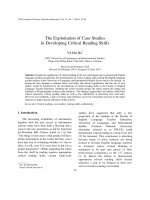
FIGURE 1. Map of the coast of California showing significant place names and undersea topograpny.
200 and 2000 m isobaths delimit shelf and slope habitat divisions, respectively.

Ine


Although it is widely recognized that seabirds
“make their living” at sea, with individuals of
many species spending more than half their lives
away from land, there exists a strong terrestrial
bias in our knowledge about characteristics and
regulation of seabird communities. Simply put,
we are only just beginning to appreciate how pattern and process in the marine environment affect these marine animals.
To a great extent this is attributable to difficulty of work at sea. While few major colony
areas in the world now are beyond the reach of
systematic study, ornithological coverage of many
ocean areas has been infrequent and unsystematic; the oceans are too large and the available
resources too limited to have permitted development of a ‘mature’ science of pelagic seabird
biology. Still poorly understood are such basic
questions as: How many seabirds species can coexist simultaneously in the same ocean habitat?
To what extent do seabirds compete with each
other for food? How closely do seabirds track
changes in ocean conditions on various time and
space scales? Do some species specialize in discrete kinds of habitat? What strategies are employed by seabirds to find suitable ocean habitat
and what environmental features serve as cues
for habitat choice? What significant life history

consequences accrue to birds making different
habitat choices? Resolution of some of these
questions would provide an informative contrast
to the body of descriptive and theoretical work
concerning population regulation through processes affecting seabirds while ashore.
Until very recently, scientific resources were
almost always inadequate to characterize the occurrence of whole marine bird faunas through
space and time. Beyond this, studies of physical

Topphoto:Sooty
California.

Shearwaters (Pujinus

by D. B. Lewis.

griseus) on Monterey

Bay,

processes and food webs seldom coincided temporally or geographically with those of offshore
bird populations. This has meant that patterns
in bird communities at sea could not readily be
explained by reference to bio-oceanographic processes. This has changed since about 1970, and
several large-scale bird studies have benefitted
from simultaneous oceanographic data collection (e.g., Ashmole 1971, Pocklington 1979,
Brown 1980, Ainley and Jacobs 198 1).
In this paper, we attempt to describe quantitatively the occurrence of seabirds in waters off
California and relate patterns of abundance, seasonality, and community diversity to physical
and biological characteristics of the ocean habitat. This is necessarily a descriptive task, one

that must precede studies focused on mechanisms and consequences of habitat choice.
Our work took place within a period of intensive oceanographic study of the California Current. Driven initially by the need to understand
the collapse of the California fishery for sardines
(Surdinopssugux),government and academic research here since 1950 has focused on processes
affecting biological productivity; until recently,
physical oceanography received less attention.
Programs supported since 1974 by the U.S. Department of Interior, Minerals Management Service, have gathered considerable information applicable to preservation of important wildlife and
habitat resources during development of offshore
oil and gas reserves. As part of that program,
researchers at the University of California undertook studies in 1975 and 1979 to assess the
status, numbers, distributions, and movements
of all seabirds in California waters. The data resulting from this and complementary work carried out by the U.S. Fish and Wildlife Service
and Point Reyes Bird Observatory now permit
a basic understanding of the ways in which seabirds use California Current habitats, how this
community is structured, and how variation in


4

STUDIES

IN AVIAN

some ocean processesaffects bird populations at
sea and on land.
We present results of standardized surveys
made with consistent methods and replicate
sampling. Our goal is to interpret distribution,
seasonality, and community organization in relation to variability in the physical environment.
This paper comprises several sections, addressing different aspects of the general problem.

First, we review the oceanography of the California Current System off California to set the
stage for later analyses of seabird habitats. Next,
the (present) status, numbers, and habitat affinities of California seabirds are discussed in the
format of species accounts. This is followed by
analyses of diversity and interspecific associations in several latitudinal/water depth regions.
Habitat use is analyzed for numerically important species using a multivariate ordination
(principal components) approach. We also describe patterns of patchiness and aggregation
among numerically dominant species and relate
these to dominant scales of variation in surface
temperature.
Ours is not the first attempt to synthesize information about the seabirds off California but
is the first to use replicate, quantitative sampling.
With Grinnell and Miller’s (1944) distributional
summary of the state’s avifauna, the general seasonality, relative abundance, and affinity for
nearshore or oceanic waters were known for most
species. The focus of the bulk of California seabird work before 1975 was the island colonies of
southern and central California (Fig. 1). Most
noteworthy is the century of ornithological investigation on the Farallon Islands (reviewed in
Ainley and Lewis 1974, DeSante and Ainley
1980) which has been continued and greatly augmented by the Point Reyes Bird Observatory.
Nesting biology of about a dozen specieshas been
studied there during the past fifteen years. Lengthy
time series of observations of nesting biology also
exist for Brown Pelicans (Pelecanusoccidentalis)
at Anacapa Island (Anderson and Gress 1983)
and for the Western Gull (Larus occidentalis)and
the Xantus’ Murrelet (Synthliboramphus hypoleucus)at Santa Barbara Island (Hunt et al. 198 1;
Murray et al. 1983). The locations and sizes of
all seabird nesting colonies throughout the state
were surveyed during 1975 to 1980 (Sowls et al.

1980, Hunt et al. 1981).
Systematic work at sea has been confined to
only a few areas. Monterey Bay has been important as a collecting locality and site for birding
trips since the beginning of the century (Loomis
1895, Beck 1910, Stallcup 1976), and the Gulf
of the Farallones has been traversed and surveyed hundreds of times en route to the Farallones colonies (Ainley and Boekelheide in press).

BIOLOGY

NO. 11

Despite the large numbers of fishing and pleasure
boats in southern California, no systematic attempt was made to document seabird numbers
and distribution in that area prior to the studies
reported here. Waters lying 50 to 950 km west
and south of Point Conception were visited about
monthly in 1966 and 1967 by personnel of the
Smithsonian Institution’s Pacific Ocean Biological Survey Program (POBSP). Results of that
program were partially reported more than a decade ago (Ring 1974), but much information remains unanalyzed in computer files or in unpublished cruise or data reports (e.g., Pyle and
DeLong 1968).
Sighting records and seasonal status of seabirds in waters off the southern California coast
were discussedby Garrett and Dunn (198 1; some
of these were based on incomplete records from
the program upon which we report). A step toward analyses of the habitat affinities of important specieswas made by Small (1974) based on
the then-available sightings from birdwatching
trips made from several southern and central
California ports. Ainley (1976) attempted to place
some (order-of-magnitude) numerical interpretation on the reports published primarily in Audubon Field Notes/American Birds (AFN/AB),
and also to relate patterns of seasonal abundance
and geographic concentration to general cycles

of ocean productivity, temperature, and salinity.
For a number of pelagic species,Ainley identified
thermal or salinity regimes that correlated with
interannual variations in bird abundance or geographic concentrations in space.
METHODS
Our resultsderive from two studiesdesignedto assessthe abundance,distribution,and habitat affinities
of all marine birds off California. From April 1975
throughMarch 1978 the watersoff southernCalifornia
were surveyedfrom both ship and airplane. Our purpose was to repeatedlysample areas of inshore and
offshore habitats with approximately monthly frequency to determine which bird species were most
abundant, the locations of preferred feeding areas, and
routes of migrations. Shipboard observers in southern
California made 24 surveys totalling more than 27,000

linear km of predeterminedtrackline.This cruisetrack
(depictedin Briggs et al. 198 lb) emphasized waters
inshore of the Santa Rosa-Co&
Ridge, which extends
for 250 km southeast of Santa Rosa Island and approximates the offshore limits of the Southern California Bight (SCB). The waters of Santa Barbara Channel were not routinely visited by our vessels, except as
part of related studies of seabird breeding biology (Hunt
et al. 198 1). Five vessel surveys reached waters of the
California Current west ofthe Santa Rosa-Corn% Ridge
during September 1975, January and October 1976,
and January and April 1977; total offshore vessel coverage was about 3 100 linear km.


CALIFORNIA

SEABIRD

Low altitude aerial surveys also were made 24 times
in southern California. Aircraft followed primarily
north-south tracks extending from the mainland to
about 200 km offshore (Fig. 2 of Briggs et al. 198 1b).
The comparatively rough waters far offshore were undersampled by aerial surveys during 1975 but were
reached routinely during subsequent years. Total aerial
coverage was about 40,000 linear km, averaging 1800
km per survey.
Surveys of central and northern California (from Point
Conception north) during February 1980 through January 1983 were conducted almost exclusively from aircraft. Monthly surveys were made along about forty
lines oriented east-west and extending up to 185 km
offshore. Initially, the lines were selected at random
from among 92 possible tracks (every 5’ of latitude)
with the stipulation that no more than two adjacent
lines would be skipped. To the initial pool of about 30
selected transects, 10 lines were added to provide more
resolution in five areas targeted for possible minerals
leasing. The between-line spacing in the final set of
transects averaged 19.8 km. Weather permitting, the
same 40 to 42 lines were then sampled each month at
least as far offshore as the base of the continental slope
(arbitrarily 2000 m). Four pairs of lines were selected
in central and northern California whereon sampling
routinely extended to 185 to 200 km from shore (these
were located at the northern edge of Santa Barbara
Channel. off Monterev Bav. off Caue Mendocino and
off Poini St. George; In practice we usually were able
to sample on four to six of these lines). This sampling
scheme led to expenditure of 40% of total sampling
effort each over waters of the continental shelf and

slope and the remaining 20% in o
‘ ffshore’ regions. Averaging about 3 100 linear km per month, total aerial
coverage was almost 83,000 km in central California
and almost 45,000 km in northern California (north
of 38”50’N; annual coverage is shown in Briggs and
Chu 1986). Six half-day aerial surveys south of Monterey Bay provided synoptic observations of offshore
populations during spring and summer 1983. Additionally, five vessel surveys were conducted in 198 1 to
determine species composition and habitat affinities of
several groups of birds off central California; 950 km
of trackline were surveyed. In all, we logged sightings
of approximately 3.5 million birds of 74 species.
OBSERVATIONPROTOCOLS
Our shipboard and aerial methods were described
and analyzed previously (Briggs et al. 1981a, 1984,
1985a, b); only a few important features will be noted
here. The aim of both techniques was to produce estimates of density (birds km-* surveyed) for each species
encountered. We sought to obtain large, replicate samples (spatially and seasonally) to facilitate statistical
analyses. Observers scanned strips parallel to the path
of the survey platform, noting lateral distance to sightings in terms of non-overlapping corridors or bands.
Ship surveys featured 400-m, bow-to-beam corridors
on each side of the vessel. Two experienced observers
attempted to minimize recounts of birds following the
vessel by noting bird numbers and identities at the
stem every 10 to 20 minutes. The southern California
ship track was divided into 106 segments, each of which
was 7.4 km (4-nautical-mile) in length and was cen-

COMMUNITIES

5

tered within a 5’ by 5’ latitude/longitude grid-cell;
wherever possible, observations were made continuously from about an hour after sunrise to an hour before
dark. Aerial observers scanned much narrower strips
(50 m) and only made observations on the shaded side
of the flight path; surveys were flown at 65 m altitude
at approximately 165 km h-l ground speed. Vessel
observers recorded sightings on prepared forms, while
those in aircraft made verbal tape recordings of similar
data. In each case, sightings consisted oftaxa, numbers,
ages or plumage morphs, behavior, associations with
other species, and environmental information. Data
taken at the start and end of each transect line included
position and time, observation conditions, environmental data, notes on observer fatigue, and reliability
of navigational information (which occasionally was
inadequate due to interference or malfunction of electronic aids).
In comparing and evaluating the strengths and weaknessesof the two methods, we found that our ship and
aerial techniques produced similar estimates of bird
density when data were matched for time and area
(Briggs et al. 1985a). Under ideal survey conditions,
aerial observers reported significantly higher densities
of birds along selected, short (to 18.5 km) transects.
However, the results of geographically broad counts
under changeable viewing conditions indicated that
density differences between the two types of platform
were not significant compared to within-sample geographic variability or variations between months. In
presenting southern California data, we emphasize the
aerial because of comparability with data taken in central and northern California. Where southern California aerial sampling included gaps of more than a month,
we have drawn from ship samples to smooth seasonal
curves, recognizing the geographic (shelf/slope) biases

in the ship track.
As might be assumed a priori, vessel surveys were
more efficient at determining the detailed species composition of bird aggregations and at identifying rare or
unusual birds. Aerial observers covered much broader
areas in relatively shorter periods, reported more sightings at the generic or family level, and noted fewer
unusual species (Briggs et al. 1985a).
SHORELINEMETHODS AND COVERAGE
Numbers of individuals at sea often represent only
a portion of a seabird population. Variable portions
may be found on land or on waters near coastal roosts
or colonies. To evaluate coastal bird numbers, we made
systematic counts of birds along most sections of the
coast, including islands, during most months (24 visits)
in southern California and quarterly (twelve times) north
of Point Conception. For the most part, this was done
by aerial observers surveying at about 100 m altitude
and 100 m away from the coast; one observer recorded
all birds on shore while another surveyed offshore to
about 200 m. Where large aggregations of birds were
known to occur (e.g., the Farallon Island nesting colonies), observations were made from as far away as
400 m altitude and 300 m setback in order to minimize
disturbance. Verbal recordings indicated locations to
within 1 km, proportions of birds on land and in the
water, and counts of each species. We made heavy use
of 35-mm aerial tele-photography. Virtually every group


6

STUDIES

IN AVIAN

of birds exceeding about fifteen individuals was photographed for later counts (from projected transparencies). This was especially important at large (1 O4to
lo5 birds) colonies and roosts where visual estimates
of numbers would only have been useful for order-ofmagnitude analyses. Where photographic quality permitted, each bird was counted on each frame. Counts
were made from more than 40,000 photographs.
To augment information for the southern California
coast, monthly censuseswere made along 18-29 beaches representing about one-tenth the length of the coast;
these included no harbors. Where we refer to these
mainland counts, we have extrapolated observed numbers by factors appropriate to the percent of the coast
covered (in linear km). These shoreline and surf censuses were made with the aid of binoculars and were
most useful for grebes, cormorants, scoters, gulls, and
terns.
ENVIRONMENTAL DATA
To determine the habitat affinities of seabirds and
to limit data quality to the best attainable, observations
of environmental conditions were made at the start
and finish of every observational watch and whenever
conditions changed. Minimally, this took place about
every twenty minutes. Observers noted wind direction
and speed, sea state, glare intensity and direction, and
presence of fog or other detriments to viewing. Sea
surface temperatures were noted at least every twentyfive minutes (approximately 7 km) using bucket or
through-hull thermometers aboard ship. During aerial
surveys ofcentral and northern California, surface temperatures were recorded at least every 9 km (minimally,
at intervals of 5’ of longitude) along tracklines by a
Barnes Precision Radiation Thermometer. This instrument, coupled to a chart recorder and calibrated
onboard against known black-body temperature, had
a nominal accuracy of ?0.2”C. Periodic overflights of

oceanographic data buoys provided additional means
of calibration.
Additional information about the distribution and
patterning of surface temperature was derived from
monthly synopses prepared by the National Marine
Fisheries Service for 1975 to 1978. bv Auer for 1980
to 1983, and from satellite-sensed ocean-temperature
images furnished by the National Weather Service and
Scripps Ocean Visibility Laboratory. Frequent, nonquantitative comparisons of these satellite images with
our in situ or remote (aerial) data assisted us in contouring of surface isotherms and in understanding the
spatial relationships between habitats.
Because of their potential importance as cues to habitat qualities and presence of food, we took special
notice along sampling tracks of occurrence of ocean
color boundaries, slicks, current or wind shears, flotsam, kelp, and feeding animals of all types. Presence
of fishing activities was noted as were apparent associations with aggregations of plankton or bait.
ANALYSES
Bird density
Transect data were recorded continuously and subsequently were partitioned geographically to permit
analyses at different scales ranging from large regions

BIOLOGY

NO.

11

down to individual sightings. To arrive at monthly
estimates of bird density, the numbers of birds observed in each 5’ by 5’ latitude or longitude segment
of ship or aerial tracks was divided by the area included
within the transect. The resulting figures, which we call

“grid cell densities,” were averaged for all samples (ship
and air, or multiple visits by the same type of platform)
taken in each location. Monthly regional mean densities derived from sample sizes (visited grid cells) ranging from 86 to 144 for the southern California shelf/
slope, and 42 to 116 for six geographic units north of
Point Conception (shelf [0 to 199 m depths], slope [200
to 1999 m] and “offshore” [> 1999 m] regions, respectively, in central and northern California). We extrapolated to estimated regional populations (approximate number of individuals) by multiplying regional
mean densities by the appropriate regional areas. Adding these estimated (“instantaneous”) regional populations for a given month provided an estimate for the
total population. In no case did we know the rates of
population turnover for migrating species. As a result,
numbers of birds actually passing through California
may have been several times larger than the “instantaneous” estimates that we present. Due to large standard errors in density estimates at sea, the error range
typical of our monthly population estimates was f 25%
to 40%. Accordingly, we report mean regional densities
(+ 1 SE) and estimated total populations, and do not
attempt to statistically assessthe significance of differences in estimates between regions or months.
Bird densities were used in two types of further analyses: they were transformed into location-specific
standing stock estimates (biomass per unit area), and
they were used along with environmental variables to
prepare matrices for principal components analyses.
Transformation of bird density to biomass density (kg
km-2) was accomplished by multiplying grid-cell densities by a figure representing mass of each species or
species group (Briggs and Chu 1987).
Species diversity
Two measures of species diversity are presented for
each area and month: the raw number of species or
groups recorded, and the Shannon Index of Diversity
(Shannon and Weaver 1949):
”

H’ = -z

(P;ln P,)
i=,

(where n is the number of species recorded and P, is
the proportion of total density contributed by species
i). Diversity indices are sensitive to scale of measurement; i.e., the size of the sampling unit affects the value
of the index. We estimated species diversity for several
(nested) scales of measurement using aerial data from
central and northern California: species lists were compiled and H’ calculated for progressively larger geographic units, starting with 5’ longitudinal (approximately 7.3 km) segments of aerial trackline. Focusing
on the central California shelf/continental slope region,
we then combined 5’ segments along 7 to 11 east-west
tracklines, each of which was about 20 to 40 km in
length (for example, all segments on the line extending
west of Point Pinos), and recalculated species numbers
and H’ for each line. Finally, we calculated diversity


CALIFORNIA

SEABIRD

COMMUNITIES

7

in central California in 1985 indicated that for several
species,aggregationshad different characteristicscales
in the two directions (Briggs et al. in press). This is
noted where it is known to occur. Becauseof this and

the apparent richness of variation on scales shorter
than could be resolved along the shelf, we limit our
discussionto cross-shelfdata.Information from southSpeciesassociationsand scalesof aggregation
em California was not included because(1) in much
We investigatedthe associationbetweenspeciesover of the region there is no clear-cut across-shelfor alongspatial scalesrangingfrom the individual flock of two
shelf orientation, and (2) topographicand island influor more birds swimming or feedingtogether,to groups enceson water circulation patterns are very complex,
of flocksseenover tens of km. These analysesrequired potentially obscuringany simple pattern in bird aggredifferent kinds of data and different kinds of statistical gations that might result from relatively simple pattools.
ternsin habitat structure.Additionally, concurrentsatThe consistencyof associationbetween specieswas ellite imagery of surfacetemperature patterns was not
estimatedby examiningsightingscomprisingmore than available for the (earlier) southern California studies,
one bird of one or more specieseither feeding together negatingthe possibility of simultaneouslyevaluating
spatialvariation in bird aggregationsand this environ(usefulprimarily for surface-foragingspecies)or swimming or flying in close proximity (up to about 50 m).
mental parameter.
Among the severalavailable indicesfor determining
To obtain meaningfulsamplesizes,theseanalyseswere
limited to specieshaving relatively high abundance.
characteristicpatch sizes in birds, we used the simple
Aerial observers frequently are unable to perceive ratio I’ discussedby Ord (1972) in preferenceto more
the structureof bird aggregationsthat extend over sev- complex, and computationally intractable measures.
eral hundred metersalong a trackline: the substructure Using bird numbers in each 3-km unit (bin) of continof a flock may be seen but cohesivenessof the whole uous aerial transects(one minute of flight time), the
unit may go unnoticed. Compared to ship observa- mean and variance were computed and the index was
tions, during which a given bird flock may be in view plotted as a function of bin size. Bird numbers were
for severalminutes (a time-sample component), aerial successivelyaggregatedinto largerbins until only three
such bins composedthe entire transect. Variations in
data are much like a singleframe out of a strip of movie
film. The result is that aerial data underestimate the I’ are consideredfor different species,locations (near
proportion of birds that associatewith one another, versusaway from active colonies), and seasons.
The 3-km unit is coarserelative to the scaleof actual
and overestimatethe proportion of non-associatedand
solitary individuals. Recognizingthis bias, we selected bird flocks.However, Schneiderand Dutfy (1985) and
only those aerial sightingspertaining to birds in as- Schneiderand Piatt (in press)have used ship data to

sociation with one another (as compared with solitary show that intensity of aggregationof a variety of seabirds) and calculatedCole’s Coefficient of Association birds is lower for bins of 1 to 3 km than for largerunits.
(Cole 1949). This index rangesfrom - 1.0 (complete Thus, while our analysis does not apply to distances
avoidancebetween two species)to + 1.O (complete as- at which birds are typically in direct visual contact,we
sociation). Significanceof the index is estimated by are able to examine intensity of aggregationover scales
correspondingto large prey patchesand different macomputinga Chi-square statistic from a 2 x 2 table in
which the cellsare: number of flockscontainingspecies rine habitats.
A and speciesB, number of flocks containing A but
not B, flocks containing B but not A, and flocks con- Habitat characteristics
taining neither.
The relationshipsof selectedbird speciesto various
We evaluatedflockassociationsby season,usingcen- environmental features were analyzed by correlation
tral and northern California data: the ‘breeding’ season and principal componentsanalyses(PCA). Values for
included April throughJuly, the ‘post-breeding’ season water temperatureand depth, distancefrom the nearest
extended from August through November, and the point of land and from the nearest point on the con‘winter’ included December through March. Approxtinental shelf-break, bottom slope (maximum elevaimately 500 to 600 flock recordswere included in each tional disparity per km) were computed for each 5’ by
seasonalanalysis.
5’ geographicgrid cell. Gradients in surfacewater temTo compare the geographicscalesof aggregationsof perature, which may help to define seabird habitats,
birds (raw numbers were used, flocks and individuals were calculated from temperature values at the cenwere treated equivalently) found on the same transect terpoint of each visited grid cell. Surfacetemperature
lines, we followed a method first applied to marine gradientswere computedastemperaturedifference(C)
bird data by Schneiderand Dufi (1985). This method divided by distancemeasuredbetween centerpointsof
employs an index of patchiness(I’ of Ord 1972) and adjacentgrid cells. Thus, a maximum of eight AT/AD
requires continuous transect data. Owing to the orivalues were available for each sampled cell, assuming
entation of our transect lines, across-shelfvariations that all neighboring cells also were sampled. We secould be resolved to about the scale of the smallest lected the maximum gradient value for each cell.
time increment routinely employed by observers(one
After major habitat components were identified by
minute of flight time or about 3 km), but patterns of PCA, we determined correlationsbetweenbird density
aggregationalong the shelf could be evaluated only at variations and valuesof habitat components.We used
much larger scale, correspondingto the interval be- orthogonal rotation of resultingaxes and a minimum
tween flight lines (9 to 28 km). Aerial and ship sampling eigenvalueof 1.Ofor inclusionin the model (SAS 1982).
from all sightingsin each region (e.g., ignoring grid
cells and transectlines and compiling a species/abundance list from all sightingsmade in May 1980 on the

central California shelf), for all of central California
(shelf, slope, and offshore) and for all of central and
northern California combined.


STUDIES

8

IN AVIAN

Bird densities were log-transformed (Sokal and Rohlf
198 1) to control variance, thus emphasizing order-ofmagnitude variations in abundance. These analyses indicated which species’ abundances most strongly correlated with variation along two or three major gradients in open-water habitats.
Our analysis of bird aggregations is complemented
by examination of the scales of variation in surface
thermal patterns. These were assessed via spatial autocorrelation, using satellite imagery obtained concurrently with sampling of bird populations. The maximum resolution of satellite data was about 1.1 km, and
values were calibrated to +0.3”C against aircraft radiometer data and against NOAA oceanographic buoy
data.
Autocorrelation analysis typically is applied to residuals rather than raw data. Thus, we sought to remove a mean trend from each data set. Regression
analysis indicated that only about 12% of variance in
satellite temperature data was explained by the pattern
of 20-year mean values for the same locations and
months (modified from Auer 1982, 1983). Although
statistically significant for the large sets of data used
(400 to 500 data points), it appeared that a better fit
to the satellite data (resulting in smaller residuals) could
be obtained by using a linear regression of temperature
against latitude and distance offshore. When this
regression was fitted to September 198 1 data, the model explained 17% of temperature variation. This procedure was adopted for de-trending data from three
additional images. After removing the mean latitude/

distance trends from the data, autocorrelations were
computed at separations of 1 to 64 km in the west and
north directions. These are reported separately for the
cross-shelf and along-shelf directions, as well as for the
combined data.
Because of the degree of processing required in computing autocorrelations from the satellite image data
and potential aliasing due to time lags (up to 24 hours)
between bird sampling and satellite imaging, we do not
attempt to statistically compare autocorrelation patterns between regions or dates. Rather, we employ these
analyses to determine whether certain bird species appear to aggregate on scales similar to those predominating in environmental data.
OCEANOGRAPHY

OF THE STUDY

AREA

The oceanography and, to a great extent, the climatology of the coast of California is dominated by
influences of the California Current, its associated
countercurrent, and by seasonal upwellings. Large scale
processesaffecting exploitable fish stocks have received
a great deal of attention over the past several decades.
Particularly well studied are the geographic and temporal variations in hydrographic parameters affecting
populations of the northern anchovy (Engraulis mordax) and Pacific sardine as well as characteristics of
plankton populations fed upon by these fish. With both
resources and research interest concentrated in waters
from northern Baja California to about Point Conception, researchers associated with the multi-agency California Cooperative Oceanic Fisheries Investigations
(CalCOFI) program have monitored physical and biological variables with mixed intensity since the late
1940s.

BIOLOGY

NO.

11

Several authors have related aspects of the physical
environment to seasonal and geographic patterns of
seabird populations and distributions in the California
Current System. Ainley (1976) drew upon existing
CalCOFI data concerning thermal and salinity regimes
off California to describe general population abundance for many seabird species in differing years, seasons, and temperature/salinity regimes. Somewhat more
detailed descriptions have appeared for several species
(Briggs et al. 1981b, 1983, 1984). Recent research and
re-examination of older information have modified
somewhat the pre- 1970 perceptions of the characteristics and processes of the California Current System.
As an update to this conceptual progress and a prelude
to habitat analyses appearing later in this paper, we
review here the oceanography of the California Current
System.
BATHYMETRY
The coastline of California trends south from Oregon
to Point Conception, then veers abruptly to the east
and southeast forming the Southern California Bight
(SCB). Major promontories include Cape Mendocino
and points Arena, Reyes, Sur, and Conception. The
continental shelf (depth O-l 99 m) is very narrow (5 to
3 5 km) in much of northern and central California, but
broadens to 50 to 75 km off Eureka, San Francisco,
and Morro Bay. Deep submarine canyons dissect the
shelf near Cape Mendocino and Monterey Bay, and

sheltered embayments are present at Eureka, Bodega,
Point Reyes, San Francisco, Monterey, Morro Bay, and
San Diego. South of Point Conception, the seafloor is
complex, consisting of a series of basins and ridges,
some topped by islands. In contrast to waters north of
Point Conception where only Aiio Nuevo, the Farallones, and Castle Rock could be considered as important island habitat, the SCB contains nine islands or
island groups (including Islas Los Coronados just
southwest of San Diego). Here, deep basins (> 1000 m)
lie close-by rugged island chains and submerged banks,
creating very complex circulation patterns. The main
continental slope runs south from Point Conception
and lies more than 200 km west of San Diego.
GENERAL CHARAC~ZRISTICSOF SURFACEWATERS
Waters off California shallower than 200 m depth
are relatively cool, fresh, and nutrient-rich compared
with those at equivalent latitudes in the central or westem Pacific, or those south of central Baja California,
Mexico. Reid et al. (1958), Hickey (1979), and Bemal
and McGowan (198 1) point out the north-south trend
in chemical and thermal conditions of surface waters:
ignoring the strong, localized, seasonal variations imposed by coastal upwellings (discussed below), waters
are coolest, freshest, and generally richest in organic
nutrients north of Point Arena. Latitudinal gradients
in temperature are greatest in late summer, when waters
off extreme northern California may be 10°C cooler
than those near the U.S./Mexico border. Sea surface
temperatures (SSTs) range between about 8 to 9°C in
the north during late winter and spring and more than
20°C near San Diego in late summer. Seasonal ranges
in temperatures and variations from twenty-year means
are presented for the waters sampled in this study by

Briggs and Chu (1986).


CALIFORNIA

SEABIRD

It is noteworthy that, beginning in about mid- 1976,
a secular rise in temperatures prevailed over all areas
and times included in this study. McLain (1983) discussed periodic fluctuations between relatively cool and
relatively warm temperature regimes in this region,
linking them to North Pacific Basin-wide shifts in meteorologic and oceanographic conditions lasting up to
a decade. A previous ‘hingepoint,’ when conditions
seemed to shift, occurred in 1957-1958.
The summer thermocline is shallower in the north
than off southern California (roughly 10 to 20 m deep
versus 30 to 60 m) and deepens with distance from
shore to more than 80 m at the seaward limits of our
study area. Phytoplankton concentration maxima often
are found at the (deep) thermocline offshore but may
peak near the surface over the shelf. Turbid waters over
the shelf result from dense plant pigment concentrations, sediment discharges from rivers and coastal bays,
and suspension of sediments by wave and current action.
Surface waters of the California Current flow in a
southerly direction, with considerable short-term, localized variability. The fastest flows are in the range
of 0.5 m see-I and center 200 to 500 km offshore. The
California Undercurrent underlies and flows in the opposite direction to the California Current through most
of the year. Its importance to bird populations and to
their prey is that the Undercurrent surfaces near the
coast from about Point Conception to at least southern

Washington from approximately November through
February. This northward coastal current, referred to
as the Davidson Current, contains water that is warmer
and saltier than California Current water at comparable
depths. In spring and summer, when the Undercurrent
flows at 100 to 300 m depth below the California Current, coastal upwelling appears to draw from the Undercurrent as replacement for surface waters that are
advected seaward.
Between the southern California mainland (south of
Los Angeles) and about 118”W, waters usually flow to
the north from about May through February or March.
Farther offshore, within the main axis of the California
Current, flow is to the southeast through much of the
year.
It is now appreciated that global and basin-wide shifts
in meteorological and hydrographic conditions associated with El Niiio-Southern Oscillation (ENSO) cycles
lead to occasional weakening of southward flow within
the the California Current, strengthening of the coastal
countercurrent in winter, and deepening and stabilization of the surface layer (0 to 300 m) density structure. In years such as 1957-1958,
1969, 1972, 1976,
and 1982-l 983, strong coastal countercurrents in winter transported warm, salty water from offshore and
south, creating a relatively stable surface layer through
which upwelling of nutrients in the subsequent spring
was impaired (Chelton 1980, McLain 1983). The profound effects of the strong 1982-l 983 ENS0 event in
California have been examined by McLain (1983),
McGowan (1984) Fiedler (1984), Ainley et al. (ms)
and others. Bemal and McGowan (198 1) and Chelton
et al. (1982) have shown that annual variations in
standing stock and productivity of plant and animal
plankton in the California Current correlate with variations in transport of water from the north. In years

COMMUNITIES

9

of strong, southward transport, primary production is
high (Smith and Eppley 1982) zooplankton standing
stocks increase, and the productivity of anchovies and
rockfish (Sebastes spp.) is at a peak. Ainley et al. (in
press) and Hodder and Graybill (1985) relate annual
changes in productivity to seabird nesting success on
the Farallon Islands and Oregon, respectively. Years
of low southward transport, particularly those with
strong ENS0 events, are characterized by low productivity in the plankton, as well as in fish and squid, upon
which most seabirds feed.
UPWELLING
Upwelling is an extremely important, localized phenomenon along the Pacific coast. Its influences are seen
not only in hydrographic characteristics ofcoastal waters
but also in various aspects of food-web productivity
and coastal meteorology. Prevalence of north- and
northwesterly winds during spring and summer leads
to offshore transport of coastal surface waters and replacement by waters drawn from depths to about 100
m. These upwelled waters are cool, salty, and rich in
organic nutrients. In addition to augmenting ocean productivity, upwellings have several characteristics of
significance to the seabird fauna. One such attribute is
the formation of strong gradients in chemical and physical properties of seawater at the seaward edges, where
upwelled waters intrude into the warmer, fresher, thermally stratified waters of the California Current. At
these ‘upwelling fronts’ (which are usually 10 to 30 km
in cross-shelf breadth), thermal gradients may exceed
0.5”C km-’ and may be accompanied by abrupt changes
in ocean color (chlorophyll fronts), slicks, accumulations of flotsom and drift kelp, and sometimes by large

concentrations of zooplankton and their predators
(Briars et al. 1984. Briars and Chu 1986. 1987). These
upwelling boundaries typically overlie the continental
slope, are structurally complex, and may persist for
several weeks. Fronts visible in satellite infrared images
extend up to 300 km along and offshore of the shelfbreak (Fig. 2).
Upwellings exert a strong influence on the composition of the prey base available to seabirds. Parrish et
al. (198 1) point out that among fishes heavily utilized
by birds for food, there exists a marked difference between the dominant species spawning in the region of
strongest upwelling (Point Conception to Cape Mendocino) and the species spawning in the SCB. For example, spawning and survival of young northern anchovies are favored by formation of large patches of
(usually dinoflagellate) prey for the larvae. These conditions frequently prevail in southern California during
late winter but are seldom seen off central or northern
California, especially (due to turbulence) in the main
upwelling season. Accordingly, anchovies do not spawn
in large numbers between Point Conception and the
California/Oregon border. In contrast, rockfishes and
flatfishes spawn in large numbers in the region of maximum upwelling and are abundant in seabird diets
through spring and early summer. Anchovy biomass,
and we assume availability to seabird predators, is
highest during spawning season in the south, and anchovies become an important component of bird diets
in central California only later in summer, after the


10

STUDIES

IN AVJAN

BIOLOGY

NO. 11

FIGURE 2. Satellite infrared image of sea surfacetemperature off California on 21 September 1981. The
coolestwaters, representedby light grey shades,are 9 to 1l”C, whereasdark shadesmark waters warmer than
16°C. Several filaments of upwelled (cool) water extend for 100s of km from major headlands (courtesy E.
Daghir).
fish undertakepost-spawningmigration out of the SCB
(see, for example, Briggsand Chu 1986, 1987).
Upwellings can occur in any season and almost
everywhere along the California coast; however, the
months of greatest extent and persistenceare April
throughabout September.Within each year, upwelling
reachesgreatestintensity earlier in the south (Nelson
1977). Peak upwelling occurs in northern Baja California from March through May, off Point Conception

April through early June, off Cape Mendocino May
through July, and off Oregon from June through late
July or early August. In all areas, favorable winds tend
to pulse; periods of heavy upwelling are interspersed
with relative calms, during which surfacewaters may
become heated by the sun and stratified, and offshore
waters may move toward the coast. Centers of upwelling, where winds are strongestand persist in directions favorable for upwelling, and where surface


CALIFORNIA

SEABIRD

waters become coolest, include Point St. George, Cape

Mendocino, Point Arena, Point Reyes, Point Sur, and
Point Arguello-Point Conception. In each of these locations, the coolest surface waters typically are found
somewhat downstream (southward and offshore) of
coastal promontories.
The general seasonality of hydrographic conditions
was characterized for Monterey Bay by Bolin and Abbott (1963). Three main seasons were the Upwelling
season (discussed above), the Oceanic season (when
upwelling ceases and thermally stratified waters originating offshore move toward the coast, bringing with
them elements of the ‘oceanic’ plankton), which lasts
roughly from late summer until November, and the
Davidson Current season (November through February) when coastal surface waters move north and coastal convergence or downwelling occurs. This scheme
has been rather loosely applied to other areas of the
state, assuming similarity of timing and conditions.
However, studies completed recently in the Point Sur
area, together with the large archive bf satellite images
of SST now available for the Pacific Coast show that
upwelling can and does occur in all seasons. At Point
Sur, Breaker (1983) found alternation of upwelling and
nonupwelling regimes. The Oceanic season of Bolin
and Abbott may in fact be peculiar to Monterey Bay
and a few other sites where large, persistent, warm
eddies of the California Current approach the coast
with the general diminution of upwelling after about
August. A warm eddy offshore of Monterey Bay can
be seen in a large portion of available satellite SST
images, but no such structure is consistently present
near Point Sur, Point Conception, Point Reyes, or Point
St. George. Conversely, large, warm eddies often approach the coast west of Eureka, near Point Arena, and
south of Morro Bay.

IMPORTANT
MESOSCALE
FEATURES
Advances in the ability of oceanographers to rapidly
assessthe hydrographic (especially thermal) and optical
characteristics of surface waters over large spatial scales
( 100s to 1000s of kms) has revealed that the California
Current System is rich in meanders and eddies. Meanders are no less prevalent in the California Current
than in more energetic western boundary currents (such
as the Gulf Stream and the Kuroshio Current) and
occur in all seasons (Hickey 1979, Huyer 1983, Mooers
and Robinson 1984). Meander effects may include current jets running counter to the southward mean flow
at speeds of up to 1.0 m sect’ (Owen 1980, Simpson
et al. 1984). The eddies studied to date have characteristic persistence scales varying with size from days
to many months; some have been shown to exert an
influence on subsurface hydrographic conditions to
depths of a few hundred meters. The most permanent
California Current eddies may be relatively fixed in
place by bottom topography.
The largest and ecologically most important eddylike structure is the so-called Southern California Eddy
which forms south and east of Point Conception and
influences hydrographic patterns through much of the
SCB. Although commonly regarded as a cyclonic recurvature of the eastern limb of the California Current
(Owen 1980), the western part of this structure appears
in satellite imagery of temperature to be a cool, ad-

COMMUNITIES

11

vetted mass contiguous with the major upwellings at
Point Conception. In contrast, waters east of the Santa
Rosa-Corms Ridge are subtropical in nature, and different from the cool waters transported away from the
Point Conception upwelling. The boundary between
these water types often lies just east of San Nicolas
Island and may in fact be a zone of strong sheer between
opposing currents. Effects of the “Southern California
Eddy” on biological populations, including important
habitat influences on spawning anchovies, are discussed by Owen (1980) and Parrish et al. (198 1).
Another mesoscale oceanographic feature of apparent significance to seabirds is the tidal plume formed
outside the Golden Gate on outgoing tides. This plume
of turbid, estuarine waters often has a very sharp edge
forming an arc extending as far offshore as 25 km into
the Gulf of the Farallones, reaching maximum expression in late winter/early spring. Waters of the plume
are less salty and of different temperature than ocean
waters of the Gulf (depending on the season, the plume
may be relatively warm or cool). Recent field studies
suggest that both plankton (euphausiid) and fish populations differ between the areas normally included
within the plume and those lying outside (S. E. Smith,
P. B. Adams pers. comm.). Aggregations of seabirds
along the edge of the plume are common, and certain
species(such as shearwaters and Cassin’s Auklets) avoid
the turbid waters of the plume itself (K.T.B., D. G.
Ainley unpubl. data).
RESULTS

SEABIRDNUMBERS AND STATUS
The California state list includes 103 species
that make up the marine avifauna. These species
obtain almost all their food from the sea and

occur on salt water more than half the year. This
total excludes the shorebirds except phalaropes,
all anseriforms except scoters and brant, and all
waders. We observed 74 marine species during
the course of our studies. About 30 of these species
were relatively numerous in their preferred habitats and seasons and accounted for the great
majority of energy cycling through the California
marine bird community (Briggs and Chu 1987).
In the following 62 species accounts we emphasize data concerning the California nesting fauna
and species whose estimated total populations
exceeded 20,000 individuals. We do not consider
species seen only once or a few times or those
never observed away from the mainland shore.
Red-throated Loon, Gavia stellata
Loons are relatively easy to identify from above
(during aerial surveys) when in the nuptial plumage (especially March through May). In autumn
and winter, however, when immature birds are
present and adults are in basic plumage, many
Pacific and Common loons (G. pacijica and G.
immer) cannot be distinguished. Red-throated
Loons (G. stellata) are always much paler, appearing small, speckled and with a slender neck.


12

STUDIES

IN AVIAN

NO. 11

BIOLOGY

\

Northern
California
c O
‘ -

\ 1
1

Olfshore

4?4
:

i ,n-

Shell-slooe

_ _ ,. ” ” ,”_ ,.,. I ” _ - ,. I .

I

1980

1981

1.._ _ I I _ _ Y I. Y,
I

lQR2

Centra II
CayjoInia

I

Offshore
g1.0

-

r 0.1
E
EQ

=

1%
.Z 10 -

I

Shelf-slope

1980

1981

1982

Southern
California
c

1

I

4

1

1975

b.LONO

“‘D
‘ ,

1976

1977

1978

FIGURE 3. Comparison of monthly mean densities of Pacific Loons in three regions off California. In t:ach

panel, three curves represent mean density i one SE. Shaded values lie more than one SE below the mean.


CALIFORNIA

SEABIRD

Where we encountered substantial numbers of
unidentified loons in winter, we arbitrarily apportioned them to species in the same ratio recorded among birds identified to species at the
same general location.
The Red-throated Loon generally is far less
numerous than the Pacific Loon and in migration
is decidedly more coastal in distribution; as with
other loons, peak numbers occur during migration and winter. There is some suggestion that
Red-throated Loons migrate a few weeks earlier
in spring and a few weeks later in fall than do
other loons.
During our studies, Red-throated Loons were
most numerous off central and northern California, particularly on the sheltered waters of
Morro Bay, Monterey Bay, the Gulf of the Farallones, and Tomales Bay, and along the open
coast from Eureka to Trinidad Head. Estimated
populations north of Point Conception were on
the order of 3800 to 16,000 in April and about
a third lessin autumn. Numbers dropped to about
2000 to 3000 in winter.
Within 0.5 km of the southern California
mainland, we found Red-throated Loons to be
more than ten times as numerous as Common
or Pacific loons. Farther to seaward, they were
relatively rare, with less than 100 seen near the

Channel Islands at the peak of winter occupancy.
Shelf waters at the eastern end of Santa Barbara
Channel harbored estimated peak numbers of
1000 to 3000 birds.
Pacific Loon, Gavia pacijica
The Pacific Loon is the most abundant and
widely distributed loon off California; the great
majority of loons seen more than about 10 km
from the mainland are of this species(Small 1974,
Ainley 1976). Because of our fixed, monthly
sampling in central and northern California, the
exact timing of the autumn migration could not
be determined. But, as was seen by DeSante and
Ainley (1980) at the Farallones, peak counts always occurred in late-November. Peak numbers
of fall migrants reached southern California in
mid-December. Relatively small populations remained in California each winter with perhaps
10,000 to 15,000 birds, on average, coastwide,
evenly distributed between northern, central, and
southern California. Populations of birds remaining through summer were very small and
concentrated from San Francisco northward.
Peak densities of Pacific Loons seen during
migrations were 0.8 to 1.8 birds kmm2 in central
and northern California and 0.4 to 1.8 birds krn2
in the south (Fig. 3). Turnover rates in migration
are unknown; however, we estimate that populations ranged from 75,000 to 287,000 at once
in central and northern California and 40,000 to

COMMUNITIES

13

60,000 in the south. Compared to these numbers,
an eleven-week spring shoreline count from Pigeon Point in central California, produced a total
of 432,000 migrating loons, 98% of which were
Pacific Loons (Winter and Morlan 1977). The
peak count of 46,770 birds came in late April
1977; these shoreline counts would have missed
a sizeable number of birds migrating more than
about 5 km from the coast.
Wintering numbers of Pacific Loons were much
smaller, with 5000 to 19,000 birds estimated for
central and northern California in January 198 1,
1982, and 1983, and about 5000 in southern
California during winter 1976, 1977, and 1978.
North of Point Conception, Pacific Loons migrated primarily over the continental shelf. During November surveys, we found more than ten
times as many Pacific Loons over shelf waters
than over the continental slope; most birds were
found from 5 to 50 km offshore. Because of the
northwest-southeast trend of the southern California coast, loons travelling southward from near
Point Conception spread over a broad offshore
area. We found them to be most common within
40 km of the southern California mainland, but
they also occurred in densities above 1.0 birds
km-2 as far offshore as 75 km. The farthest offshore that we saw Pacific Loons was 110 km west
of Monterey and at Tanner Bank, 165 km southwest of Los Angeles (but only 65 km south of
San Nicolas Island).
During winter, Pacific Loons occupied only
relatively sheltered waters along mainland and
island coasts; favored sites included Bodega and
Tomales bays, the Gulf of the Farallones, Monterey Bay, and eastern Santa Barbara Channel

(where densities occasionally rose to over 80 birds
krne2 over the shallows northeast of Anacapa
Island). The 300+ km stretch of coast north of
Point Arena, where winter storminess is most
severe, harbored only about 5% of the statewide
winter total.
Spring migration took place in March through
early June with a distinct peak at the time of our
late-April counts. DeSante and Ainley (1980)
noted a peak in late March at the Farallones, but
our larger samples consistently indicated a later
peak for central California. The pattern of spring
migration looked like that in fall, except that we
frequently saw hundreds or thousands of loons
feeding or resting in shallow waters of the island
passes of Santa Barbara Channel. Loons in
breeding plumage occurred among them as late
as 15 June (1975 and 1976).
Common Loon, Gavia immer
We noted migrating Common Loons from late
March to late May and late October to midDecember, but data were too sparse to detect any


14

STUDIES

IN AVIAN

seasonal peak or north-south trend in timing.

DeSante and Ainley (1980) noted that peak migration dates at the Farallones were late October
to mid-November.
Extrapolation from densities recorded in five
April surveys (1976, 1977, 1980, 1981, 1982)
suggests that the i‘nstantaneous’ population of
Common Loons was between 5000 to 10,000
birds at sea and about 1000 within 0.5 km from
the coast. Common Loons were concentrated near
the coast at Morro Bay, Monterey Bay, the Gulf
of the Farallones, Tomales Bay, and north of
Trinidad Head (the same areas as the Redthroated Loon), but undoubtedly were still more
abundant on estuarine waters not included in our
samples (e.g., San Francisco Bay).
This species was difficult to identify during
winter aerial censusesof the coastline; however,
Common Loons appear to have numbered less
than 1000 statewide from December through
March.
Eared/Horned

Grebe,

Podicepsnigricollis/auritus
Due to their narrow along-coast distribution
and a tendency to dive at the approach of aircraft,
small grebes (predominantly Eared Grebes, but
also Homed Grebes) were difficult to identify and
not adequately censused by our aerial survey
techniques; in this account we refer to them collectively as Eared Grebes, noting that Homed
Grebes probably accounted for less than 5% of

all small grebes seen on open coastal waters. Ship
surveys around the southern California islands
provided reliable counts, but not all islands were
visited each survey, and the mainland was not
censused in this way.
Eared Grebes were sighted near the Santa Barbara Channel islands from September through
June each year, with high counts in January or
February (2834 were counted in February 1976).
Along the mainland of southern California we
saw far fewer birds; populations along the open
coast were as low as 500 to 1000 birds during
winter. Numbers throughout southern California
dwindled for a month or two in late winter, then
rose again in midspring, apparently as a result
of birds moving into the area from the south
(Eared Grebes are abundant in the Gulf of California through April; D. W. Anderson and K.T.B.
unpubl. obs.). We counted up to 1800 small grebes
during winter aerial surveys of central and northem California, most within Tomales Bay and at
the entrance to San Francisco Bay; this figure
may understate the actual numbers of these grebes
present in the region by one or more orders of
magnitude. Flocks of hundreds of Eared Grebes
are seen during winter in the vicinity of the Farallon Islands; an estimated 3 120 birds occurred

BIOLOGY

NO. 11

there during fall and winter 1974-l 975 and peak
counts were attained from mid-December

through mid-March (DeSante and Ainley 1980).
Western/Clark’s

Grebe,

Aechmophorusoccidentalis/clarkii
These two species were not distinguishable
from the air and Clark’s was not yet given species
rank at the time of our southern California studies. For simplicity we collectively refer to both
species as “Western” Grebes.
The Western Grebe is one of the predominant
species in waters within 0.5 km of the mainland
coast during October through May, and at least
a few birds can be found on inshore waters
throughout the year. This speciesshows a distinct
preference for waters over sandy bottom lessthan
10 m deep (determined from coastal charts and
direct observations from the air), especially
downwind from major headlands.
Up to a few hundred birds appeared on saltwater in central and northern California by late
September each year. Numbers of birds on coastal waters increased throughout fall, and peak
populations occurred from November through
January. Winter numbers were variable, probably reflecting movements to and from coastal
estuaries in response to the passage of storms. A
coastwide decline in numbers was seen after
March, and populations were lowest from May
through late August (Fig. 4).
Because Western Grebes occupied an extremely narrow band, within about 0.5 km of the
coast, their numbers were poorly resolved by our
offshore transects. Along-coast counts were relatively infrequent, and suspected weather-related population movements render even this technique somewhat inadequate. However, peak

populations were on the order of 25,000 birds
north of Point Conception and 27,000 to the
south. Three areas of concentration in winter were
evident: the coast from Trinidad Head to Point
St. George, which was usually occupied by 4000
to 5000 birds; the waters from Bodega Bay to
Monterey Bay, which harbored up to about
10,000 birds; and the shallows at the eastern end
of Santa Barbara Channel, which supported an
estimated 2000 to 27,000 birds (averaging 10,000
on three January surveys). Counts along the coast
in summer were much lower: 1700 to 4100 in
central and northern California during July 1980,
198 1, and 1982, and perhaps 500 to 800 along
the southern California coast during 1975 to 1977.
Western Grebes were very uncommon offshore,
even near island shores. They were scarce near
the Channel Islands, and DeSante and Ainley
(1980) have reported that fewer than ten birds
occur at any given time at the Farallones. Interestingly, at the Farallones, these grebes reached


CALIFORNIA

SEABIRD

1981

1980

COMMUNITIES

15

1982

FIGURE 4. Shorelinecountsand open-waterdensitiesof Western/Clark’s Grebes. (A) Shorelinecountsof
grebesin northern California (open bars) and centralCalifornia (solid) during 1980-l 982. (B) Mean densityof
grebesin shelfwatersof centraland northernCalifornia (combined).(C) Estimatedgrebepopulationsthroughout
southernCalifornia extrauolatedfrom mainland and island beachcountsand aerial transectsof easternSanta
BarbaraChannel.
-

peak numbers in late September and
tober and were much less numerous
(DeSante and Ainley 1980) a pattern
ferent from that characteristic of the
coast.

early Octhereafter
quite difmainland

Black-footed Albatross, Diomedea nigripes
The Black-footed is the most numerous albatross on coastal waters of the U.S. Pacific coast
and is present throughout the year. Peak abundance occurred from May through July, with an
estimated 15,000 to 75,000 birds present in early
summer. Numbers were lowest from October
through February, during which period we estimate a population totalling only 500 to 1500
birds.
Various authors have commented on latitudinal patterns in Black-footed Albatross abundance and seasonality off California. Sanger

(1974), analyzing observations gathered during
100 months of sampling by the CalCOFI program during the 1950s showed a strong northsouth gradient in numbers: Black-footed Albatross were two to ten times more abundant north
of Point Conception than to the south. In central
and northern California, Sanger detected no obvious east-west trend, but off southern California
albatrosseswere more numerous far offshore (i.e.,
in the California Current proper) than within

about 100 km of the coast. These observations
were based on counts made while ships were on
station for hydrographic work, and coverage was
quite variable between months and regions. Ainley (1976) examined accounts published in AFN/
AB and also suggested that Black-footed Albatross were more numerous in central and northem California and less so farther south. He noted
that the peak in sightings occurred later off southem California (August) than off central California (May-July).
Our data, which are based on replicated coverage in all seasons, show three trends with regard to seasonal distribution of this species: 1)
In almost all cases, densities were much higher
north of San Francisco than to the south (Fig. 5);
2) birds were more numerous over the continental slope than either the shelf or the waters farther
to seaward (we did not sample some of the regions far offshore discussed by Sanger 1974); and
3) there was a northward seasonal withdrawal of
the center of abundance from April onwards.
Birds were concentrated north of San Francisco
in all seasons,but in summer, at peak population,
the largest numbers of birds were seen north of
Cape Mendocino.
Off southern California, we noted peak numbers in May or June each year. By far, the largest
portion of the 7 1 sightings there occurred within


STUDIES

16

IN AVIAN

NO. 11

BIOLOGY

Northern
Zalifomla
.
-i

?

lo1.0-

ONshore

lo-

Shell-slope

1980

A

1981

!

1982
\

\
c

:entral
:alifgnia
c

1.0 -

b
ii

10’

\

Oflshore

1

1
1980

1981

1982

i

Southern
California
CT

E

f
$

lo, o _

Shelf-slope

FIGURE 5, Comparison of monthly mean densities of Black-footed Albatross in three regions off California.
In each panel, three curves represent rnem density ? one SE. Shadea values lie more than one SE below the
mean.


CALIFORNIA

SEABIRD

25 km of the axis of the Santa Rosa-Co&s Ridge,
especially near San Miguel Island and TannerCortCs Bank. These are the coolest and most productive waters off southern California. We think
that the late-summer peak in sightings reported
by Ainley (1976) is a function of seasonal and
geographic bias in data from birdwatching trips

originating at southern California ports: in spring
and early summer these trips usually avoid the
rough, cool, offshore waters where albatrosses
actually concentrate.
Black-footed Albatross were most numerous
along the upper continental slope from the Farallones to Eureka. Within these areas occur some
very complex and dynamic interactions between
upwelling filaments and warm, California Current eddies (Huyer and Kosro 1987). Albatross
generally were found on the warmer, more translucent sides of color or thermal boundaries separating these two types of water. These areas also
support important trawl fisheries that provide
considerable quantities of fish offal to scavenging
albatross.
Our southern California data are insufficient
to ascertain much about interannual variability
in numbers, but fewer birds were sighted in 1976,
an ENS0 year, than in 1975 or 1977. In central
and northern California, numbers of Black-footed Albatross were 50% lower at the 1982 June
peak than in the two previous years. And, densities were comparatively low from July 1982
onward. At about this time, oceanographers were
noting atmospheric changes relating to the onset
of the intense 1982-1983 ENS0 episode. Sanger
(1974) noted a similar decline in albatross numbers in central California coastal waters during
the 1957 episode; farther offshore the pattern was
not obvious.
Laysan Albatross, Diomedea immutabilis
We saw Iaysan Albatrosses infrequently off
central and northern California and rarely off
southern California. Thirty-three sightings of
single birds were logged in central and northern
California; all but two (August 1982) were seen

in November through April, and all but five were
north of Monterey Bay. We saw one Laysan at
Co&s Bank in January 1976, and six or more
during an April 1977 cruise in the California
Current off southern California (from 121” to
122”W). Most birds were seen over deep water
seaward of the shelf.
Northern Fulmar, Fulmarus glacialis
Fulmars occurred off California in all seasons,
but large numbers were seen only from October
through March or April. We found that fulmars
usually entered the area from the north in October and became abundant off southern Cali-

COMMUNITIES

fomia after about mid-November. In all regions,
populations built to a late fall-early winter peak
(November, December, or January north of
Monterey, and December or January south of
there), then dropped to a midwinter low, usually
in February (Fig. 6). There followed another
(lower) peak in abundance in March, then numbers dwindled through spring. We interpret this
pattern to indicate movement through California
of birds that winter off Mexico; the low in winter
corresponds to the period when many birds are
south of California or far offshore.
Extrapolations from regional density data indicate that combined, statewide populations
reached about 225,000 to 360,000 birds in December-January, while only 35,000 to 95,000
birds were present at the winter low. In most
months, fulmars attained highest densities at sea

between Point Pinos and Bodega Bay. With little
annual and regional variation, dark or mediumplumaged birds accounted for two-thirds or more
of all birds for which plumage morph was noted
(n = 1043 in 1975-1978 and 998 in 1980-1983).
Northern Fulmars were decidedly most numerous in waters seaward of the middle of the
continental shelf (5 to 40 km from the mainland),
and were recorded as far offshore as we surveyed
(to 460 km, June 1982). Fulmars also were seen
close to the mainland shore; in November 198 1,
about 200 fulmars were observed at Santa Cruz
(Monterey Bay) feeding in the surf zone on the
carcass of a juvenile sperm whale (Physeter catodon; W.B.T. unpubl. obs.).
Ainley (1976) noted a correspondence between
large numbers of fulmars and periods of cool
temperatures and high surface salinity. This general pattern helps to explain certain variations
in numbers observed during our studies. During
winter, fulmars were much more common in the
cool waters west of the southern California islands than in the warm waters nearer the mainland. As the incidence of upwelling increased
there during spring and early summer, the fulmars remaining off southern California concentrated in the coolest upwellings near Point Conception and San Miguel Island and avoided the
warmer coastal waters to the southeast. Fulmars
were about three times more numerous off southem California in 1975-1976, a cool-water winter, than in the warmer winter of 1976-1977.
Off central and northern California during
winter, Northern Fulmars concentrated seaward
of the zone influenced by freshwater runoff from
land. After most birds departed in March and
April, remaining birds shifted toward the coast
and concentrated in upwelling centers (cool and
saline water) during spring and early summer.
Additionally, fulmars occupied the relatively
warm neritic waters between Point Conception

STUDIES IN AVIAN BIOLOGY

18

lorthern
:alifornia

1981

1980

1982

:entral
:alifomia
.

1u

Offshore

,.

i

1980

1981

1982

\

\

Southern
California

1975

1976

1977

1978

FIGURE 6. Comparison of monthly mean densities of Northern Fulmar in three regions off California. In
each panel, three curves represent mean density + one SE. Shaded values lie more than one SE below the mean.


CALIFORNIA

SEABIRD

and Monterey Bay in large numbers during the
cool winter of 1980-l 98 1 but not in the warmer
winters before and after. Further, on a larger scale,
during the onset of ENS0 conditions in fall 1982,

fulmars were confined to a cool-water zone lying
seaward of a wedge of warm water that was narrow (25 km) at Cape Mendocino but broader
than 200 km off central California. In thermal
satellite imagery it appeared that the habitat of
the fulmar was w
‘ edged’ offshore by strong northward coastal currents emanating from south of
Point Conception.
After winters of high fulmar abundance (1976
and 198 l), some birds lingered off California
throughout summer. We recorded at least a few
birds on every survey in both years, almost all
near sites of upwelling (Point Conception, Point
Reyes, Point Arena, and Cape Mendocino).
In light of these observations, we interpret the
apparent large variations in prevalence of fulmars off California as reflecting regional redistributions of a population that may not vary tremendously in size between years (except in the
extreme case of the 1982-1983 El Niiio). Fulmars were present in greater numbers near the
coast in years when waters were cool and salty.
In other years, they remained offshore beyond
the reach of single-day bird-watching trips.
Gadfly Petrels, Pterodroma spp.
The status of Pterodroma petrels in waters off
the U.S. Pacific coast is very poorly known. Three
species have been identified in recent years and
a fourth may have occurred but could not be
clearly separated from the others. Mottled Petrels (P. inexpectata) occasionally move into California waters from the west during late winter
(Ainley and Manolis 1979). These are thought
to be non-breeders or failed breeders migrating
from nesting areas in the southwestern Pacific to
the Gulf of Alaska. Solander’s Petrel (P. solandri)
is known from sightings of about twenty individuals 65 to 110 km off Cape Mendocino to

Point Reyes in May 1981 (R. L. Pitman pers.
comm.). Additionally, Cook’s Petrel (P. coo&i)
has been seen a few times during warm-water
periods in summer and autumn, mostly off the
coast of San Luis Obispo County. A single specimen record for this speciesexists for the Pacific
coast: a live individual was recovered from a
beach in Santa Cruz in November 1983 (Tyler
and Burton 1987).
On the basis of typical dorsal plumage patterns
and soaring flight characteristic of this genus, we
considered eleven birds seen off central and
northern California to be Pterodroma petrels. Ten
of these occurred in late winter or spring (March
through June) and the other in November. All
were seen well offshore of the shelfbreak in scat-

COMMUNITIES

19

tered locations. In June 1985, three Pterodroma
were seen in 14°C waters within 75 km seaward
of the Farallones (D. G. Ainley, R. Ferris, and
K.T.B. unpubl. obs.). Thus, these petrels probably occur each year seaward of the coastal upwelling zone.
Pink-footed Shearwater, Pufinus creatopus
Pink-footed Shearwaters nest along the southwestern coast of South America and visit California during the northern summer. We found
that Pink-footed Shearwaters and Sooty Shearwaters (P. griseus)often occurred in mixed species
flocks off California, but the two speciespursued
somewhat different patterns of seasonal habitat
occupancy, The Pink-footed was about 10% to

20% as abundant as the Sooty on a statewide,
average basis, but within its favored habitat, it
was often the more numerous species.In contrast
to the Sooty, the Pink-footed Shearwater was
distinctly more abundant off southern California
than offcentral California (and was still lesscommon north of Point Arena).
Extrapolations of density values indicate that
maximum numbers were reached in May through
August or September, with peak populations of
around 130,000 offcentral California and 60,000
to more than 400,000 off southern California.
Population curves for southern California were
bimodal each year, with May or June peaks followed by midsummer lows and later peaks in
August or September. In 1977 the September
peak was higher than that in the preceding spring,
while in 1975, the reverse was true. Off central
California, density curves for Pink-footeds were
essentially unimodal in two years, with gradual
build-ups to September peaks followed by abrupt
October declines (Fig. 7). In 1982, however, when
ENS0 conditions were becoming established in
the eastern tropical Pacific, we recorded an early,
low population peak in May and June, an abrupt
decline in July, and a second, lower peak in August and September (the bimodal pattern usually
seen to the south).
Off central and northern California, we observed Pink-footed Shearwaters from near the
shore to about 150 km at sea; numbers were
much higher over the continental shelf and upper
continental slope than farther offshore. The shelf
areas from Point Reyes to Monterey Bay and

from Morro Bay to Point Argue110supported the
largest and most consistently occurring concentrations. Off southern California, Pink-footed
Shearwaters were most common in Santa Barbara Channel, near the southern coasts of the
northern island chain, and along the Santa RosaCortCs Ridge. Like the Sooty, these shearwaters
preferred the cooler, shallow regions of the
Southern California Bight. Outside the seasons


STUDIES

20

Northern
California
c O
‘ 3

IN AVIAN

BIOLOGY

NO. 11

\
!‘
Olfshore

1-

l.O-

A

Shelf-slope

Central
California
10 -

$-1.0
9
e
3

b
p

\
Olfshore

-

0.1 A

0

1

Shelf-slope
lo-

Southern
California
2

Shelf-slope

1978

1977

1978

FIGURE 7. Comparison of monthly mean densities of Pink-footed Shearwater in three regions off California.
In each panel, three curves represent mean density + one SE. Shaded values lie more than one SE below the
mean.