Evaluating intangible asset using panel data applying for vietnam listed companies
Bạn đang xem bản rút gọn của tài liệu. Xem và tải ngay bản đầy đủ của tài liệu tại đây (1.67 MB, 66 trang )
UNIVERSITY OF ECONOMICS
INSTITUTE OF SOCIAL STUDIES
HO CHI MINH CITY
THE HAGUE
VIETNAM
THE NETHERLANDS
VIETNAM - NETHERLANDS
PROGRAMME FOR M.A IN DEVELOPMENT ECONOMICS
BY
LAI THANH BINH
MASTER OF ARTS IN DEVELOPMENT ECONOMICS
HO CHI MINH CITY, DECEMBER 2014
A thesis submitted in partial fulfilment of the requirements for the degree of
MASTER OF ARTS IN DEVELOPMENT ECONOMICS
By
LAI THANH BINH
Academic Supervisor:
Dr. LE VAN CHON
HO CHI MINH CITY, DECEMBER 2014
2
This research tends to investigate the effect of intangible assets to company’s
performance. In this research, some of methodology to evaluate sum of intangible
assets will be represented and panel data will be used in model estimation. All firms
used in practical examination are chosen from 250 Vietnam listed companies standing
for different industries. Firms in industries could use these results to allocate
investment on sum of all intangible assets other than just constructing new factories or
opening new brands.
Estimation shows that intangible asset take a huge proportion on total company
asset. Intangible asset not only take an important part in the past performance but also
explain their role as the key factor of future development. When interpreting
relationship among kinds of asset and firm’s value, we recognize that intangible asset
significantly impact on firm’s added value, however it do not show a clarify
relationship with firm’s stock price. Reason comes from fluctuation of stock market
and some external factor affecting to stock price.
3
ABBREVIATION
M&A: Merger and Acquisition
R&D: Research and Development
IAS: International Accounting Standard
EBIT: Earning Before Interest and Tax
CAPM: Capital Asset Pricing Model
GSO: Vietnam General Statistics Office
WTO: World Trade Organization
SBV: State Bank of Vietnam
WACC: Weighted Average Cost of Capital
4
TABLE OF CONTENTS
CHAPTER 1. INTRODUCTION ............................................................................ 9
1.1.
Problem Statement ......................................................................................... 9
1.2.
Research Objective ...................................................................................... 10
1.3.
Research Questions...................................................................................... 11
1.4.
Structure of Thesis ...................................................................................... 11
CHAPTER 2. LITERATURE REVIEW .............................................................. 12
2.1.
What Are Intangible Assets ......................................................................... 12
2.2.
Types Of Intangible Assets ......................................................................... 12
2.3.
Intangible Asset Valuation Approaches ...................................................... 14
2.3.1.
Cost Approach ...................................................................................... 14
2.3.2.
Market Approach .................................................................................. 15
2.3.3.
Income Approach .................................................................................. 15
2.3.4.
Panel Data Approach ........................................................................... 16
2.4.
Conceptual Framework................................................................................ 17
CHAPTER 3. ECONOMETRIC MODEL ........................................................... 18
CHAPTER 4. EMPIRICAL RESEARCH............................................................ 22
4.1.
Data Sources ................................................................................................ 22
4.2.
First estimation: Calculate α and β .............................................................. 25
4.2.1.
Consumption ......................................................................................... 30
4.2.2.
Banking ................................................................................................. 34
4.2.3.
Steel Industry ........................................................................................ 37
4.3.
Estimate Cost Function ................................................................................ 40
4.4.
Compute Firm’s Equity Value ..................................................................... 42
4.5.
Compute Firm’s Equity Value with Non Intangible Asset ......................... 44
4.6.
Evaluating Firm’s Intangible Asset ............................................................. 45
4.7. Examine Relationships among Firm’s Revenue, Intangible Asset and
Tangible Asset ....................................................................................................... 45
5
4.8.
Firm’s Intangible Asset and Policy Implications ........................................ 51
CHAPTER 5. CONCLUSION ............................................................................... 59
REFERENCE......................................................................................................... 65
6
LIST OF TABLES
Table 1: Category of Intangible Asset ........................................................... 13
Table 2: Categorized Intangible Assets ......................................................... 22
Table 3: Result of equation 5 using fixed-effects and random-effects model27
Table 4: Hausman test .................................................................................... 27
Table 5: Testing for heteroskedasticity using Wald test ................................ 27
Table 6: Testing for multicollinearity using VIF index ................................. 28
Table 7: Effect of Industry on Firm’s Output ................................................ 28
Table 8: Estimation with all variables............................................................ 48
Table 9: Effect of intangible asset and industry development on firm’s added
value ................................................................................................................ 48
Table 10: Effect of intangible asset on firm’s added value ........................... 49
Table 11: Association among intangible asset, tangible asset, industrial
growth rate and stock price. ............................................................................ 50
Table 12: Association between tangible asset and stock price ...................... 50
Appendix 1: Fixed effect estimation without industrial dummy variables ... 61
Appendix 2: Random effect estimation without industrial dummy variables61
Appendix 3: Random effect estimation with industrial dummy variables .... 61
Appendix 4: Random effect estimation with industrial dummy variables after
adjusted heteroskedasticity ............................................................................. 62
7
LIST OF FIGURES
Figure 1: Relationship between distribution channel and business of Masan
Group ........................................................................................................... 34
Figure 2: Steel scrap price in period from April 2008 to December 2014 . 38
Figure 3: Amazing performance of Hoa Sen Group .................................. 40
Figure 4: Change of total factor of production (TFP) ................................ 46
Figure 5: Ratio of Intangible asset on Total asset ...................................... 47
8
CHAPTER 1. INTRODUCTION
1.1. Problem Statement
The fantastic merger and acquisition (M&A) stories of famous Vietnam brands
make a lot of financial researchers actually confuse. According to Kinhtedautu
magazine (April 2014), foreign companies bargained these acquisitions at unexpected
price, more higher than total tangible assets of these companies, such as Phở 24 (about
20 million dollar) or ICP (higher than 60 million dollar). These businesses raised a
question about original source of firm’s intrinsic value. Firms are unable to fully
evaluate benefit of intangible assets or misunderstood about importance of devoting
money on invisible assets. Because of these distortions, calculation about operation
efficiency and payback period of project or firms could be inaccurate. For instant,
brand is one of intangible asset and it could make firm’s product sell at higher volume
with higher price. If analysts do not evaluate strength of brand, he could get stuck in
some problem with forecasting future revenue.
There are some reasons why intangible assets have to be correctly evaluated. One of
these reasons is about unstable characteristic of economy and it is the most important
information not only for company’s management board but also for investor’s
decision. Companies always change themselves, from operating activities to
expanding activities, to appropriate with market, if they don’t want to narrower their
market share and to lower their income. However, general financial statement might be
unable to tell us all of company’s effort to change their business. According to a
research of Baruch Lev and Paul Zarowin (1999), our current report-system such as
balance sheet, income statement or cash flow statement deteriorated their usefulness
over the past several years. A lot of money spends on R&D activities or advertising
were not be showed on these statement and just record as expense. Secondly,
economic situation changes day by day and the firms will hard to keep their customers
buying their product if it does not create any interesting thing. By this reason, spending
money on intangible asset seems to allocate fund on innovative activities. Finally, if
9
companies couldn’t appropriately assess value of intangible asset, they might be
violated matching concept in accounting standard. Each earned revenue need to
suitable with expense creating it.
In addition, valuating intangible asset used to apply on some important sectors
including financial reporting, commercial strategy and strategy for development. It
come to financial purpose, shareholders do concentrate on company’s financial
position and corporation’s expectation. When these factors could be presented clearly,
shareholder will be more loyalty with company and cost of equity could be lower also.
Beside financial purpose, some intangible assets such as brand or intellectual capital
also help firm create differential rate of return via increasing customer loyalty and
creating differential margin on sale (according to Parble Fernandez (2013)). A famous
brand can sell their product at higher price and reduce their cost by negotiating price of
input with suppliers. In sense of strategy development, according to Mike Rocha
(2014), manager of company could plan their investment strategy, how much for
factory constructing and what proportion for marketing…
After all, demand for measuring value of intangible assets is very clear.
Furthermore, finding an appropriate method places an important role in intangible
asset research. As Parble Fernandez (2013) said, we are just at the begin point on the
way to evaluating intangible assets. Up to now, there are three methods to calculate
total value of these assets. This research will apply a new method to do this job.
1.2. Research Objective
Specially, this research measures magnitude of intangible asset effect on company
performance in different industries. This result will help firms decide to allocate their
resources in different kind of asset. New method, indirect approach using panel data
method, will be used to calculate total value of intangible assets for Vietnam selected
companies.
10
This thesis also solves another objective related to development policies. It rises a
problem about supporting policies between small and medium enterprise (SME) and
larger companies.
1.3. Research Questions
Base one research objectives above, this research will solve two questions:
Why should companies allocate their resources in both tangible and
intangible assets?
What policies control market power of both SME and large companies?
1.4. Structure of Thesis
The study will consist of four main components, include: literature review,
conceptual framework, econometric model and empirical study. The first section will
present the preliminary studies of previous authors on the subject of intangible assets.
In this section, we will go through the different approaches to evaluate intangible
assets. The strengths and weaknesses of each method will be analyzed in detail,
thereby, highlighting the advantages of T.Yamaguchi (2014). The second part explains
the improvement in model of Yamaguchi paper, and generalizes the idea that makes
the valuation method of the author. Next, evaluation process will be visualized the
diagram in section two. In part about econometric model, it will raise qualitative
methods used in the study and interpretation of the calculation method. This section
will interpret specific econometric model is applied in the study. The final section
expresses the process applying the evaluation method of intangible assets for
businesses in Vietnam stock market. The specific calculation is applied to illustrate the
value of intangible assets for each business and each industry. Section 4 also studies
the relationship between intangible assets affect the performance of the business.
11
CHAPTER 2. LITERATURE REVIEW
2.1. What Are Intangible Assets
Because of different perceptions about intangible assets, so that definition about
them also different. In accounting point of view, prudent concept keeps definition
about these assets more rigorous. Besides that, in investor or manager point of view,
they will assess and define intangible asset broader.
According to International Accounting Standard Board, Standard 38 (IAS 38)
defines an intangible asset as: "an identifiable non-monetary asset without physical
substance." Besides that, this standard also requires future certain economic benefit as
an important characteristic of intangible asset.
According to OECD project (2011), with a different perspective, OECD defines
“intangible assets are assets that do not have a physical or financial embodiment”. In
addition, OECD also identifies the difference between intangible asset and intellectual
asset. Base on OECD definition, intellectual assets are a part of intangible asset.
Besides that, intangible asset include three different: “computerized information”;
“innovative property”; “and economic competencies".
In this research, we will follow OECD’s definition to estimate aggregate value of
intangible asset. It means that we will use the word “intangible asset” instead of
“intellectual property” or “intellectual asset”. This definition allows us not to have
problem with matching concept and undervaluation of current financial reporting
system.
2.2. Types Of Intangible Assets
There is a lot of way to categorize intangible asset. Researchers usually separately
study kinds of intangible assets such as brand name, lists of customers, company’s
atmosphere .etc. One of these intangible asset categories is paper of Petros A.
Kostagiolas and Stefanos Asonitis (2009). They listed types of intangible assets as
below:
12
Table 1: Category of Intangible Asset
13
Source: P.A.Kostagiolas and S.Asonitis (2009)
Despite of a lot types of intangible assets, this research just concentrate on effect of
total intangible asset on company’s income. However, understanding categorizing of
intangible assets will use to choose Valuation approach and help to interpret root of
industrial growth rate in later sections.
2.3. Intangible Asset Valuation Approaches
According to the book Valuing Intangible Assets of Reilly, R. F., and Schweis, R. P.
(1999), these are three approach to evaluate intangible asset, include cost approach,
market approach and income approach. Each approach uses different data sources and
has to go through a lot of procedures. In addition, each approach also includes
different methods and creates a range of reasonable value of intangible assets. Usually,
researchers only apply one of these valuation approaches due to limitation of collected
information and cost of collecting data.
2.3.1. Cost Approach
According to Lev and Sougiannis (1996), cost approach evaluate intangible asset
base on total amount of money to recreate this intangible asset or to build a similar one
which has the same function. Lev and Sougiannis interpret value of R&D activities in
relationship with company’s earning. To examine this relationship, authors have to
calculate value of intangible asset, and they solve it base on total cost spend on the
past R&D activities. This method might record an accurate value of some intangible
assets such as R&D expense or advertising expense. However, it is actually difficult to
value other intangible assets such as brand name, staff’s experience or lists of users.
On the other hand, determining the useful life of intangible assets is an actual
14
challenge because it is repeatedly examined to find out suitable lag term of R&D
expense affecting operating earnings.
2.3.2. Market Approach
Market approach appraises value of intangible asset by market price of a similar
asset which is selling on the same market. In a paper of Kossovsky (2002), market
approach were used to indirectly determine value of intellectual assets base on
different between book value and market value of firm’s equity. This approach could
objectively measure value of intangible asset due to compare with market price of
company. Nevertheless, price of company’s stock reflects not only current intrinsict
value but also shareholder perception about future of firm’s prospective. In addition,
sometime, stock price also distort by temporary speculation. Furthermore, if appraiser
estimates value of intangible asset depending only on a comparable asset, this
approach couldn’t implement if appraiser is not able to find out any similar asset. In
reality, it is essentially hard to identify two similar intangible assets.
2.3.3. Income Approach
Income approach gauges value of intangible asset base on extreme benefit between
having intangible asset situation and disappearing intangible asset situation. More
clearly, intangible asset value equal subtraction between net present values of two cash
flows in these situations.
Interbrand’s valuation method is one of income approach based on methods used to
calculate brand’s worth. They calculate different earning associating with a new
variable, brand’s strength. However, Paulo Fernandez showed some problems related
to Interbrand’s method in his paper, Valuing intangible asset and intellectual property
(2013). First, Interbrand identifies extreme benefit of intangible asset by difference of
EBITs between a famous brand and a private label company. The problem is how to
determine private label company? Because private label company is the firms which
don’t have any market power from their brand name, it is obviously hard to recognize
15
this factor. Second, with Paulo Fernandez, the procedures to calculate brand’s strength
are subjective and it could be manipulate by appraisers.
2.3.4. Panel Data Approach
The panel data approach bases uses panel data analysis to compute invisible firmeffect. Unobservable firm effects were interpreted in Motohashi (2005) as
management ability, labor’s motivation and R&D expense. Even though, because
R&D expense could be exactly identified, Motohashi added it as an independent
variable in his model. Motohashi’ method used components in production function to
examine effect of labor, capital and internet network on firm’s value added. However,
in this model, Motohashi just interprets internet network effects, other intangible assets
are parts of error term. He also recommended estimation using cross-section data, fix
effect and random effect.
Ramirez and Hachiya (2006) presented other method, used fix effect to calculate
value of intangible assets. He used sale growth rate as explained variable and some
production factors as explaining variable such as R&D expense, sale and general
administrative expenses. This method still relate to market value of firm and might be
biased as market approach, although it began with production function and used
production factors.
Other method using panel data is research of Sadowski and Ludewig (2003). In this
paper, authors used added value as explained variable instead of market value of
equity. Explainatory variable included capital and labor, human capital and social
capital. In paper of Tomohiro Yamaguchi (2014), panel data also use and intangible
assets will be measured by firm’s fixed effects. His paper differs from previous
research due to method to value company’s assets. This method will use both
production function and cost function to gauge firm’s added value with and without
intangible asset.
16
2.4. Conceptual Framework
Production Function
Calculate α and β in production
function
Cost Function
Equity of firm
Equity of firm
withour
Intangible Asset
Subtract
Intangible Asset
Book Value of Equity
Tangible Asset
Firm’s
Added
Value
Through the studies, we found that each study was caught in specific matters.
However, study of T.Yamaguchi (2014) provided a more reasonable approach when
using panel data and indirect approaches to solve the limitations of the previous
studies. His research went through many intermediate calculations to come to the
intangible value of the company. First, production function and cost function were
used as origin of calculations about firm’s equity. Then, he calculated the equity of
firm excluded the impact of intangible assets. Finally, value of intangible assets was
got from enterprise’s value minus total value of firm’s tangible assets. This approach is
more practical and indirect method based on relizable data. It eliminates speculative
assumptions about future economic value of intangible value. The final step to check
the scope of intangible assets is the regression about relationship between enterprise
value (revenue or stock price) and kinds of asset. According to the results, we could
evaluate the importance of intangible assets with businesses.
17
CHAPTER 3. ECONOMETRIC MODEL
This research bases on Tomohiro Yamaguchi’s method to calculate value of
intangible assets. After that, it will examine effects of these assets on firm’s added
value (and value of firm’s equity) in comparison with tangible assets.
The formula of growth of company is based on Cobb and Douglas production
function (1928):
𝛽
𝑄
𝑄𝑖𝑡 = 𝑎𝑖 𝐾𝑖𝑡𝛼 𝐿𝑖𝑡 𝑒 𝜀𝑖𝑡 (1)
Where: 𝑄𝑖𝑡 is added value of firm i in year t,
𝐾𝑖𝑡 stands for capital of firm i in year t,
𝐿𝑖𝑡 is labor of firm i in year t.
The parameter 𝑎𝑖 in equation 1 indicates effects of total factor productivity (TFP).
These factors include advantage of internet using, power of buyer, power of seller,
intellectual capital, staff’s motivation .etc. In total, they are effect of intangible assets
on company’s growth rate. However, growth rate of company’s value not only base on
firm’s total assets but also changing firm’s value overtime (Hulten, 2000). By this
reason, intangible asset effects 𝑎𝑖 include firm-specific effects 𝐴𝑖 and growth rate λ of
industry h in time t.
𝑀
𝑄
𝛽
𝑄𝑖𝑡 = 𝐴𝑖 𝑒 ∑ℎ λℎ𝐷ℎ(𝑖)𝑡 𝐾𝑖𝑡𝛼 𝐿𝑖𝑡 𝑒 𝜀𝑖𝑡 ,
Where:
ℎ = 1, … , 𝑀
(2)
λℎ presents growth rate λ of industry h
𝑀
𝑎𝑖 = 𝐴𝑖 𝑒 ∑ℎ λℎ𝐷ℎ(𝑖)𝑡
𝐷ℎ (𝑖) is dummy variable of firm i in industry h.
𝐷ℎ (𝑖) = {
1 𝑖 𝜖 𝑉ℎ
0 𝑖 ≠ 𝑉ℎ
To estimate this function, we have to take logarithm form of equation 2. According
to T.Yamaguchi (2014), he replaced β by 1-α to make equation less complicated. To
do this replacement, his paper assumes that the researched companies have constant
18
economies of scale. However, in this paper, αand β will be estimated separately to
study aggregate market with assumption that we could bot primarily identify type of
economic of scale.
𝑀
𝑄
𝑙𝑛𝑄𝑖𝑡 = 𝑙𝑛𝐴𝑖 + ∑ λℎ 𝐷ℎ (𝑖)𝑡 + 𝛼𝑙𝑛𝐾𝑖𝑡 + 𝛽𝑙𝑛𝐿𝑖𝑡 + 𝜀𝑖𝑡 (3)
ℎ
The ith firm’s added value is directly calculated from its financial statements,
starting at operating profit. The firm’s value added includes depreciation and personnel
expense and operating profit. In addition, firm’s added value has also to remove from
effect of inflation, since, firm’s added value will be used in deflator form.
𝑝𝑡 𝑄𝑖𝑡 = 𝑂𝑝𝑒𝑟𝑎𝑡𝑖𝑛𝑔 𝑃𝑟𝑜𝑓𝑖𝑡 + 𝐷𝑒𝑝𝑟𝑒𝑐𝑖𝑎𝑡𝑖𝑜𝑛 𝐶𝑜𝑠𝑡 + 𝑃𝑒𝑟𝑠𝑜𝑛𝑛𝑒𝑙 𝐸𝑥𝑝𝑒𝑛𝑠𝑒𝑠 (4)
With pt is deflator in year t.
Because value of sum of intangible assets is achievement of this research, we are
not able to regress equation 3 without value of 𝐴𝑖 . The first step will be estimation of
equation 3 to get two parameters αand β. We will take difference form of variables in
this equation and expectation of 𝑙𝑛𝐴𝑖 will be zero, fixed effects will be extracted.
𝑀
𝑑 (𝑙𝑛𝑄𝑖𝑡 ) = ∑ λℎ 𝐷ℎ (𝑖)𝑑 (𝑡 ) + 𝛼𝑑 (𝑙𝑛𝐾𝑖𝑡 ) + 𝛽𝑑(𝑙𝑛𝐿𝑖𝑡 ) + 𝑑(𝜀𝑖𝑡𝑄 ) (5)
ℎ
Where d(…) is difference form of variables.
Because firm’s added value includes cost of production factors, we couldn’t
compute value of company by discount just firm’s added value flow. Instead, we will
use company’s profit.
= Operating Profit – Interest Rate – Tax (6)
= 𝑝𝑡 𝑄𝑖𝑡 – (Depreciation Cost + Personnel Expense + Interest + Tax) (7)
We also have the firm’s total cost C excluding cost of goods sold:
𝐶 = 𝐷𝑒𝑝𝑟𝑒𝑐𝑖𝑎𝑡𝑖𝑜𝑛 𝐶𝑜𝑠𝑡 + 𝑃𝑒𝑟𝑠𝑜𝑛𝑛𝑒𝑙 𝐸𝑥𝑝𝑒𝑛𝑠𝑒 + 𝐼𝑛𝑡𝑒𝑟𝑒𝑠𝑡 + 𝑇𝑎𝑥 (8)
So that, firm’s profit is available to compute via formula:
𝜋𝑖𝑡 = 𝑝𝑡 𝑄𝑖𝑡 − 𝐶𝑖𝑡 (9)
19
Cost of company will be identified base on duality approach which is a principal
concept in microeconomics to approach for production function and cost function, and
has been debated by Samuelson (1947), Shephard (1953, 1970), Uzawa (196) etc. In
duality approach, a certain product could be manufactured by combining production
factors at which manufacturer ensures that cost is minimized. Cost function will be
estimated follow production function.
−1/(𝛼+𝛽)
𝛼 𝛽/(𝛼+𝛽)
𝛽 𝛼/(𝛼+𝛽)
𝛼
𝛼+𝛽
𝐶𝑖𝑡 = [𝐴𝑖 𝑒
∑𝑀
ℎ λℎ 𝐷ℎ (𝑖)𝑡
Where
𝑅𝑖𝑡 is nominal cost of capital of firm i in year t
]
(
𝛽
+
𝛼
𝛽
𝛼+𝛽
) 𝑅𝑖𝑡 𝑊𝑖𝑡
1
𝛼+𝛽 𝜀 𝐶
𝑖𝑡
𝑄𝑖𝑡 𝑒
(10)
𝑊𝑖𝑡 is nominal wage of firm i in year t
We will calculate cost function through equation 10. After that, firm’s added value
𝑄𝑖𝑡 and α, β will be obtained from estimating equation 5.
̂
̂
̂
𝛽
̂ /(𝛼
̂ +𝛽 )
𝛼
𝛼
̂
̂
1
1
− ̂ 𝛼
𝛼̂ 𝛽/(𝛼̂+𝛽) 𝛽̂
̂
̂
̂
̂
̂
+𝛽
𝛼
+𝛽
̂
𝛼
𝛽
̂
𝛼
+𝛽
) (𝑎̂𝑖 𝛼̂ 𝛽̂ )
𝐶̂𝑖𝑡 = (
+
𝑅𝑖𝑡 𝑊𝑖𝑡 𝑄̂𝑖𝑡 𝛼̂+𝛽̂ (11)
𝛼̂
𝛽̂
Next step, equity nominal value of equity Eit , which containing effect of intangible
assets, will be estimated from net present value of two flows, firm’s added value flow
and firm’s total cost flow.
𝑝𝑡 𝑄𝑖𝑡 𝑒 λℎ 𝐶𝑖𝑡
𝐸𝑖𝑡 =
−
(12)
𝑟𝑖 − λℎ
𝑟𝑖
Where:
𝑝𝑡 is deflator
𝑟𝑖 is cost of equity of firm i in year t
However, 𝐸𝑖𝑡 includes value of intangible assets. To compute value of intangible
assets, we will subtract value of tangible asset from 𝐸𝑖𝑡 . Nominal value of equity
without intangible assets 𝐸𝑖𝑡𝑛𝑜𝑛𝐼 will be obtained by below formula:
𝛽
𝐸𝑖𝑡𝑛𝑜𝑛𝐼
𝛽
𝑝𝑖 𝐾𝑖𝑡𝛼 𝐿𝑖𝑡 (𝛼𝛽)(𝑅𝑖𝑡𝑛𝑜𝑛𝐼 )𝛼 (𝑊𝑖𝑡𝑛𝑜𝑛𝐼 )𝛽 𝐾𝑖𝑡𝛼 𝐿𝑖𝑡
=
−
(13)
𝑟𝑖
𝑟𝑖
20
Where:
𝑛𝑜𝑛𝐼
𝑅𝑖𝑡
is nominal cost of capital without intangible assets.
𝑊𝑖𝑡𝑛𝑜𝑛𝐼 is nominal wage of labor without intangible assets.
𝑛𝑜𝑛𝐼
𝑅𝑖𝑡
and 𝑊𝑖𝑡𝑛𝑜𝑛𝐼 are able to be identified by:
𝛽
𝑅𝑖𝑡𝑛𝑜𝑛𝐼
𝑝𝑖 𝐾𝑖𝑡𝛼 𝐿𝑖𝑡 𝑟𝑖 − λℎ
= 𝑅𝑖𝑡
(14)
𝑟𝑖
𝑝𝑡 𝑄𝑖𝑡 𝑒 λℎ
𝑊𝑖𝑡𝑛𝑜𝑛𝐼
𝑝𝑖 𝐾𝑖𝑡𝛼 𝐿𝑖𝑡 𝑟𝑖 − λℎ
= 𝑊𝑖𝑡
(15)
𝑟𝑖
𝑝𝑡 𝑄𝑖𝑡 𝑒 λℎ
𝛽
From equations 12 and 13, we could calculate value of intangible assets 𝐼𝑖𝑡 by the
difference between 𝐸𝑖𝑡 and 𝐸𝑖𝑡𝑛𝑜𝑛𝐼 .
𝐼𝑖𝑡 = 𝐸𝑖𝑡 − 𝐸𝑖𝑡𝑛𝑜𝑛𝐼 (16)
From equation 16, we could interpret proportion of intangible assets in firm’s total
asset. Base on this result, we will compare intangible asset effect and tangible assets
effect on firm’s market value and firm’s performance.
𝑀
𝑌𝑖𝑡 = ∑ λℎ 𝐷ℎ (𝑖)𝑡 + 𝑐1 𝑇𝑖𝑡 + 𝑐2 𝐼𝑖𝑡 + 𝜀𝑖𝑡 (17)
ℎ
Where:
𝑇𝑖𝑡 is value of firm’s tangible assets,
𝑌𝑖𝑡 is firm’s stock price or firm’s added value.
21
CHAPTER 4. EMPIRICAL RESEARCH
4.1. Data Sources
This research will be conducted for Vietnam listed companies in different
industries. These are 214 chosen companies and data are collected from 2008 to 2012.
We chose this time range to lower effect of economic recession from previous period.
Table 2: Categorized Intangible Assets
Rit
Wit
Firstly, firm’s operating profit multiplying deflator stands for firm’s added value.
This data could be calculated through equation 4. There are some researches
estimating Cobb-Douglas model which use different proxies for firm’s added value.
Hsing and Yu (1996) used value added to represent for output. On the other hand, B.
Lev and S. Radhakrishnan (2003) refer revenue to proxy for output. In a research
about intangible asset, T. Yamaguchi (2014) used earning before tax, depreciation and
amortization to stand for output. In this research, EBIT will be used to represent output
because it contains added value after subtract value of raw inputs. Components to
calculate equation 4 will be collected from VEC database include account TS131,
TS132, TS161, TS162 (depreciation); TN11 (personal expense); KQKD8, KQKD12
(operating profit).
22
Secondly, Capital K and Labor L could be collected from VEC database. According
to B. Lev and S. Radhakrishnan (2003), net plant, property and equipment (PP&E)
stand for capital K. Account of construction in process does not included because this
unfinished asset could not be used to make profit currently. It come to labor, they use
number of labor in firm to present labor component. T. Yamaguchi (2014) used the
same data of labor and capital as B. Lev and S. Radhakrishnan’s research. Based on
these papers, this research will do one more calculation in which total expense for
labor will stand for L. The number of labor more appropriately presents effect of labor
factor to firm’s added value when Cobb-Douglas function is in derivative of logarithm
form. In the other words, this approach is suitable to interpret change of labor factor
and capital factor in relating to EBIT. In this research, K and L in Cobb-Douglas
function were also used to evaluate equity values, so that it will be more appropriate to
use total expense of labor instead of number of labor. Data related to K and L will be
collected from some accounts in VEC database including TS11, TS12 (capital K);
LD11, LD13, TN11, TN12 (labor L).
It comes to nominal cost of capital R; it will be calculate from Capital Asset Pricing
Model. Calculating firm’s rate of return (r) is the first step before compute R. “r” is the
return that common shareholders expecting firm’s operations could create, it is also
called as cost of equity. This rate of return is different from nominal cost of capital R;
because R is weighted average among capital flows include equity, debts, and
liabilities. Calculating firm’s rate of return is a challenge due to uncertain future cash
flow. We are unable to exactly forecast future inflow and outflow of company because
they always fluctuate in term of amount and timing. To solve this problem, we could
use one of the common approaches such as capital asset pricing model, the dividend
discount model, and the bond yield plus risk premium method. In this research, we
will use the first one, capital asset pricing model.
23
Base on CAPM approach, William Sharpe (1964) find out expected firm’s rate of
return from relationship between risk-free rate and premium from bearing the stock’s
market risk (beta*(rm-rf)).
𝑟 = 𝑟𝑓 + 𝑏𝑒𝑡𝑎 ∗ (𝑟𝑚 − 𝑟𝑓 )
With:
𝑟 is firm’s cost of capital,
𝑟𝑓 is risk-free rate,
𝑟𝑚 is market rate.
Risk-free rate could be collected from risk-free assets that almost have no default
risk. Treasury bond or government debt instrument is the common proxy for risk-free
asset. The problem now is which kind of bond is appropriate for calculate firm’s rate
of return. In general, we will select risk-free rate of Treasury bond which has the same
duration with firm’s stock. However, basing on accounting assumption about goingconcern, firm’s stock has infinitive duration, so that we will use a long-term treasury
bond, ten years bond, to stand for risk-free asset.
In term of risk premium, we have to realize and cover all risks in this component
such as inflation, business cycle, credit risk and so on. One of researches try to capture
multiple-risk is the three factor Fama-French model (Fama & French, 1992).
However, the historical equity risk premium approach is the good indicator to estimate
risk premium using data observed over long period. This method calculate risk
premium via historical data of average country’s market return and risk free rate of this
country. The most important requirement for database is that collecting period need to
enough to cover almost economic cycle, both expansion phase and recession phase. In
paper of Dimson, Mask and Stauton (2003), they used this method to compute risk
premium for 16 countries, include United State over period 1900-2002. This paper
show transparent result of equity risk premium relative to Treasury Bond and help
reader more understand about existing of risk premium.
24
In this research, historical equity risk premium approach will be used to calculate
equity’s risk premium. However, we need to deeply understand some limitations of
this method. The first limitation is that stock index always changes, so that, return of
stock market fluctuates over time. The second limitation is unstable risk aversion of
investors. Finally, historical period cover of the data is also one of limitation. Despite
these limitation, this approach still prove it appropriation overtime and was employed
by a lot of researchers. Finally, IFS database will be used to get deflator data for
studying years.
4.2. First estimation: Calculate α and β
We will use equation 5 to determine α and β. Before regressing to this equation,
form of data would be taken derivative. The difference of this regression is large
number of company in three industry categories. It is actually hard to sort and process
time series data of listed companies following their tax ID number. I used both SPSS
and Excel to solve this problem. In the first step, necessary data will be gathered and
categorized in some industries. The next step, each firm will be taken derivative
separately and be created dummy for company’s industries. After having derivative
form of K, L, Q and dummy variable D (we have 50 industries so that the number of
dummy variable is 49), equation 5 could be conducted.
According to T. Yamaguchi (2014), panel data fixed-effect model will be applied to
regress equation 5 after conducting Hausman’s test. We will use Hausman test in this
research to compare efficiency between fixed-effect and random-effect model. After
taking Hausman’s test, result show that fix-effect model will be more appropriate.
Cross-section in this model will be firm level, because we could not make the same
industry ID and the same time period. After that, industrial dummy variable will be
added to test effect of industry growth rate on firm’s performance. To regress this
equation with industry’s dummy variable D, T.Yamaguchi used Panel Least Square
Method with Fixed Effects Model. In this research, we will test relationship among
added value and other input include capital, labor, industrial growth rate using fixed
25