The effects of foreign bank entry, deregulation on bank efficiency in vietnam
Bạn đang xem bản rút gọn của tài liệu. Xem và tải ngay bản đầy đủ của tài liệu tại đây (1.31 MB, 63 trang )
UNIVERSITY OF ECONOMICS
HO CHI MINH CITY
VIETNAM
ERASMUS UNVERSITY ROTTERDAM
INSTITUTE OF SOCIAL STUDIES
THE NETHERLANDS
VIETNAM – THE NETHERLANDS
PROGRAMME FOR M.A IN DEVELOPMENT ECONOMICS
THE EFFECTS OF FOREIGN BANK ENTRY,
DEREGULATION ON BANK EFFICIENCY
IN VIETNAM
BY
LUONG CONG HOANG
MASTER OF ARTS IN DEVELOPMENT ECONOMICS
HO CHI MINH CITY, November 2017
UNIVERSITY OF ECONOMICS
HO CHI MINH CITY
VIETNAM
INSTITUTE OF SOCIAL STUDIES
THE HAGUE
THE NETHERLANDS
VIETNAM - NETHERLANDS
PROGRAMME FOR M.A IN DEVELOPMENT ECONOMICS
THE EFFECTS OF FOREIGN BANK ENTRY,
DEREGULATION ON BANK EFFICIENCY
IN VIETNAM
A thesis submitted in partial fulfilment of the requirements for the degree of
MASTER OF ARTS IN DEVELOPMENT ECONOMICS
By
LUONG CONG HOANG
Academic Supervisor:
PHAM DINH LONG
HO CHI MINH CITY, November 2017
2
DECLARATION
“I certify the content of this dissertation has not already been submitted for any
degree and is not being currently submitted for any other degrees.
I certify that, to the best of my knowledge, and help received in preparing this
dissertation and all source used, have been acknowledged in this dissertation.”
Signature
Luong Cong Hoang
Date: November 10th, 2017
i
ACKNOWLEDGEMENT
Foremost, I would sincerely thank Dr. Pham Dinh Long, my supervisor, for his great
support and advice in this thesis.
Furthermore, I would like to thank the Vietnam –Netherlands Program, especially
professor Truong Dang Thuy and staffs for their assistance in this thesis.
I also would like to thank all my friends who always standing beside me with
encouragement.
Lastly, I would like to thank my family for their great support not only in this thesis
but also in my life.
ii
ABSTRACT
This study examines the effects of foreign banks entry to the efficiency of Vietnam‘s
domestic banks following the government to initiate deregulation its financial
banking. We also review the bank efficiency in term of bank size and ownership
structure. There are two principled approaches to assess the efficiency of a bank by
data envelopment analysis (DEA) and stochastic frontier analysis (SFA) methods. In
this paper, we apply the SFA method which is suggested by Berger et al. (2009), Ahn,
Lee & Achmidt (2001) to estimate the cost and profit efficiency of three groups that
includes 100% foreign-owned, big four state-owned and other domestic banks. Based
on the initial sample which is collected from the BankScope database from Bureau
van Dijk and FitchRatings and also annual reports of 37 banks in Vietnam over the
period of 2009 to 2015. Results indicate that big four state-owned banks are seemly
efficiency on both cost and profit approach while the 100% foreign-owned banks are
not the most efficiency overall. However, the 100% foreign-owned banks are able to
gain economy of scale in revenue while the big four state-owned and other domestic
banks hardly take an advantage of economic of scale. All group of bank obtain the
diseconomy of scope but the level is different.
Key words: foreign banks entry; financial deregulation; bank efficiency; data
envelopment analysis (DEA); stochastic frontier analysis (SFA); economy of scope;
economy of scale.
iii
LIST OF ABBREVIATIONS
DEA
Data envelope analysis
SFA
Stochastic Frontier Analysis
SFM
Stochastic Frontier Model
MLDV
Maximum likelihood dummy variable
SBV
State bank of Vietnam
SOCBs
State-owned commercial banks
JSCBs
Joint stock commercial banks
CE
Cost efficiency
PE
Profit efficiency
TFE
True fix effect
TRE
True random effect
TE
Technical efficiency
AE
Allocative efficiency
EE
Economics efficiency
NPLs
Non-performance loans
LDR
Loan to deposit ratio
CAR
Capital adequacy ratio
iv
TABLE OF CONTENTS
DECLARATION .................................................................................................................. i
ACKNOWLEDGEMENT................................................................................................... ii
LIST OF ABBREVIATIONS ............................................................................................ iv
CHAPTER 1: INTRODUCTION....................................................................................... 1
1.1.
Problem statements ..................................................................................................... 1
1.2.
The evolution of Vietnam’s banking sector ................................................................ 3
1.3.
The research objective ................................................................................................ 7
1.4.
Organization of the thesis ........................................................................................... 7
CHAPTER 2: LITERATURE REVIEW .......................................................................... 8
2.1.
The theoretical literature ............................................................................................. 8
2.1.1.
Theory of productivity and efficiency..................................................................... 8
2.1.2.
The method of efficiency measurement ................................................................ 12
2.1.2.1.
Data envelope analysis (DEA) .......................................................................... 12
2.1.2.2.
Stochastic frontier analysis (SFA) ..................................................................... 14
2.1.3.
2.2.
Economy of scope and economy of scale ............................................................. 17
Empirical studies....................................................................................................... 19
2.2.1.
Vietnamese researches .......................................................................................... 19
2.2.2.
International research of foreign bank efficiency ................................................. 21
CHAPTER 3: DATA AND METHODOLOGY ............................................................. 24
3.1.
Research methodology .............................................................................................. 24
3.2.
Data descriptions....................................................................................................... 29
CHAPTER 4: RESULTS AND DISCUSSION ............................................................... 32
4.1.
Descriptive statistics ................................................................................................. 32
4.2.
Regression results ..................................................................................................... 37
4.3.
Discussion ................................................................................................................. 43
CHAPTER 5: CONCLUSION ......................................................................................... 48
REFERENCES................................................................................................................... 50
v
LIST OF TABLES
Table 1: Laws of domestic banks and foreign banks ..................................................4
Table 2: A snapshot of Vietnamese Banks in 2015 (bil VND)...................................7
Table 3: An overview of development of SFA’s method .........................................16
Table 4: Data sample over the period 2009-2015 .....................................................29
Table 5: Overview of the variables of cost and profit function. .............................31
Table 6: summary statistics of variables in period of 2009-2015 .............................32
Table 7: Market share of total assets, 2009-2015 (%) ..............................................34
Table 8: The mean value of ROA, ROE, 2009-2015. ...............................................37
Table 9: The loan-to-deposit ratio, 2009 – 2015 (%) ................................................37
Table 10: Mean value of cost and profit efficiency, 2009–2015. .............................37
Table 11: Mean value of the measured overall cost efficiency, 2009-2015. ............39
Table 12: Mean value of the measured overall profit efficiency, 2009-2015. ..........39
Table 13: The economy of scope for three groups of bank: 2009 - 2015 .................41
Table 14: The economy of scale of banks: 2009 - 2015 ...........................................43
Table 15: Net interest income and non-interest income, 2009-2015. .......................44
vi
LIST OF FIGURES
Figure 1: Structure of banking system in Vietnam .....................................................4
Figure 2: Economic efficiency following input approach ........................................10
Figure 3: Economic efficiency following output approach ......................................11
Figure 4: Economic of scale from the cost approach ...............................................18
Figure 5: The stochastic production frontier .............................................................25
Figure 6: Market share of total assets, 2009-2015 (%) .............................................35
Figure 7: The ratio of total cost to total assets ..........................................................35
Figure 8: Return of assets (ROA)..............................................................................36
Figure 9: Return of equity (ROE) .............................................................................36
Figure 10: Cost and profit efficiency based on time-variant specification ...............38
Figure 11: Cost and profit efficiency, 2009-2015. ....................................................39
Figure 12: Cost efficiency, 2009-2015. ....................................................................41
Figure 13: Profit efficiency, 2009-2015. ...................................................................41
Figure 14: The economy of scope, 2009-2015. ........................................................42
Figure 15: Number of branches, 2016. ....................................................................47
vii
CHAPTER 1:
INTRODUCTION
Problem statements
Banks are notable institutions in any society since they importantly contribute to the
1.1.
development of the economics system. Via operations, banks connect the surplus and
deficit capital economic agents. Due to the power of financial intermediation of
banking industry, there are many empirical studies with the goal to enhance the bank
efficiency and stability. There have been many changes in the business environment
in recent years. Because of the boom of economics, globalization, deregulation and
technological innovation. This leads to the competitive pressure and instability of
banks industry.
Rosengard & Du (2009) describes financial deregulation as the transition from a
closed to a competitive financial system. To more specific, with banking system, it
means that the transfer of bank from monopoly or oligopoly, where have a restriction
on competition, bank entry, expansion, and diversify, to an open and more
competitive in banking system. The government make an effort to create “a level
playing field” not only between privately owned banks and public sector banks, but
also between foreign banks and domestic banks.
This paper examines the impact of bank deregulation on Vietnamese banking
efficiency. We consider which bank efficiency has improved after financial
deregulation. Instead of comparing the consequence of deregulation with the
consequence of without deregulation, we evaluate the performance of Vietnamese’s
domestic banks by using the outcome of foreign banks as the benchmark. In line with
Claessens et al. (2001) believed that in developing countries like Vietnam, foreign
banks were more efficient than the domestic banks. Therefore, it is reasonable to
assume that foreign banks have got a superior governing structure and organization,
skilled labor force and technical innovations. No previous research in Vietnam uses
a set of data including foreign banks before.
1
Farrell (1957), who is the first person introducing the theory of efficiency. He clarified
3 kinds of efficiency: technical efficiency (TE), allocative efficiency (AE) and
economics efficiency (EE). A bank has been seen as efficiency when they have
obtained a maximum level of outputs from a given group of inputs or obtained a given
level of outputs from using less than the minimum inputs (technical efficiency); and
allocative efficiency, which estimates the ability of the bank to treat inputs in optimal
ratios given their prices. The economic efficiency is reflected by the multiplication
of allocative and technical efficiency. In the literature, we may measure the cost and
profit efficiency as the duel of the economic efficiency. To more specific, the cost
efficiency estimates how to minimize the cost to achieve a given level of outputs.
Based on the cost function that total costs depend on an amount of outputs, price of
inputs, inefficiency and error term. In meanwhile, the profit efficiency analysis
measures how to attain the maximum achievable profit with a given level of inputs.
It may be similarly estimated as the cost function by changing some variables.
Following the previous research, there are two main approaches to assessing the
efficiency of banks, data envelope analysis (DEA) and stochastic frontier analysis
(SFA). The first, founded by Charnes, Cooper, and Rhodes (1978), DEA is a nonparametric technique applying the linear programming technique to set the best
practices. The second, in meanwhile, developed by Aigner et al., Meeusen and Van
den Broeck (1977), SFA is a parametric technique which distinguishes the residuals
from an estimated function into a stochastic error term and an efficiency. Instead of
using the DEA approach, we apply the SFA estimation procedures suggested by
Berger et al. (2009), Ahn, Lee & Schmidt (2001), Good &Sickles (1995), Schmidt &
Sickles (1984). We estimate the cost and profit efficiency depend on a given inputs
and outputs factors of foreign, big four and other domestic banks. Based on the dataset
from Bankscope (Bureau van Dijk) and some missing value has been collected by the
annual report of 37 banks for the post-WTO period of 2009-2015, we find that foreign
banks are not the most efficiency overall but big four is seemly efficiency on both
cost and profit approach. We also discuss the reasons behind this results.
2
1.2. The evolution of Vietnam’s banking sector
Bank industry is perceived both an opportunity access to modern technologies for
enhancing market efficiency, and the challenge amid increasingly fierce competition
from financial deregulation. This mean that the transition from a banking monopoly
or oligopoly, where constraint of competition, market entry, expansion, and
diversification, to an open and competitive banking system.
Before 1945, Vietnam was a feudal-colonial country under the French
colonialists’ rule. The banking and credit system namely Indo China bank was
established to serve the French colonialists.
During the period of 1945 – 1986, the Vietnam’s banking system had
functioned as a mono-banking model and had not been market-oriented (Siregar,
1999). At that time, the State Bank of Vietnam (SBV) was playing as a government’s
budget tool, a vehicle for government policies by supplying fiscal resources to the
State and financing for State Owned Commercial Banks (SOCs). All financial
transactions had been controlled through SBV which functioned both as a central
bank and as a commercial bank.
However, after the Sixth National Congress of the Communist Party in 1986,
the banking system of Vietnam was transformed from one-tier into two-tier.
Specifically, SBV primarily acted as a central bank which responsible for limiting
monetary policy and managing commercial banks. The banking operations such as
currency trading, forex, payment, credit and banking services in line with law are be
conducted by the commercial banks and credit institutions.
3
Figure 1: Structure of banking system in Vietnam
The State bank
of Vietnam
State-owned
commercial
banks
Joint-stock
commercial
banks
Foreign banks
(Source: the State Bank of Vietnam, 2016)
The main purpose of this reform is to diversify ownership, enhance private
monitoring, improve stability and maximize competition. To more specific, the
authorization of JSCBs (Joint Stock Commercial Banks) was established in the 1990s
and foreign banks have been licensed to participate in a type of branches or joint
ventures with domestic banks.
However, the government conducted some laws which were further restrict foreign
banks entry in term of products, a possibility of operations and registered capital.
Table 1: Laws of domestic banks and foreign banks
Domestic banks
Registered capital: No less
Requirements
for
establishment
Foreign banks 100%
-
than 3000 billion VND for
all
commercial
banks.
Registered capital no less
than 3000 billion VND
-
At least 10 billion US
(According to Decree No.
dollars in total assets in
141/2006/NĐ-CP)
previous year
-
The capital adequacy ratio
must exceed 8%.
4
Domestic banks
Foreign banks 100%
-
The ratio of NPLs is lower
than 3% at the previous
year.
-
Positive profit at least 3
years previous.
Make loans, take deposits,
business
Line of business
credit
insurance
card,
-
Same as domestic banks
-
The
agency,
settlement of accounts, bill
acceptance.
The
loan-deposit
ratio
loan-deposit
(LDR) is less than 90% (Big
(LDR)
four); 80% (other domestic
(Government
banks).
No.36/2014/TT-NHNN)
(Government
No.36/2014/TT-
-
less
ratio
than
90%
Circular
Asset and
Circular
The ratio of loans to a single
liability
NHNN)
borrower is less than 15% of
management
The ratio of loans to a single
its total equity
borrower is less than 15% of
its total equity
Reserve
Meet
the
legal
deposit
requirements
reserve requirement set by
-
Same as domestic banks
-
9% (Government Circular
SBV
Minimum
9% (Government Circular
capital
No.36/2014/TT-NHNN)
adequacy
ratio
(CAR)
5
No.36/2014/TT-NHNN)
After WTO entry in 2007, Vietnam conducted a series of financial deregulation with
the purpose of enhancing the efficiency and stability of the banking system.
Related to WTO commitments, Vietnam government issued the decree No
22/2006/NĐ-CP to allow a typical foreign institutional investor owning a 15% shares
in a domestic bank. However, a maximum of 30% shares in a particular domestic
bank to be owned by all foreign holdings. Further, the foreign institutional investor
can be categorized as “strategic” investors. Thus, they can increase their shares in a
particular domestic bank from 15% to 20%. Besides, it was the first time 100 percent
foreign-invested banks have been allowed in Vietnam from April 1, 2007. To be
precise, HSBC Vietnam is the first foreign bank which set up a wholly- owned foreign
bank in early 2009. From 2009 to 2017, Vietnam consists of seven foreign banks with
100 percent foreign-invested, namely HSBC (Hong Kong), ANZ (Australia), Shinhan
(South Korea), Standard Chartered (UK), Hong Leong (Malaysia), Public Bank
(Malaysia) and Woori Bank (South Korea).
The next deregulation is bank ownership diversification. It means that the
privatization has been highly supported by the government. The central bank
encourages transforming state ownership to private ownership. Following the
Government for Notice No.03/TB-VPCP declared that the state ownership has been
decreased by 49% by 2010.
The competition between banks has a dramatic improvement since 1990s. As
the number of joint stock commercial banks increase from 4 in 1991 to 51 in 1997.
In fact, the rapid change also increased an instability such as cross-ownership, an
increase in NPLs. To strengthen the stable bank industry, some new laws have been
conducted by SBVs via mergers and acquisition, a bank restructuring. Consequently,
the number of domestic banks declined from 42 to 34 in the period of 2006 – 2015.
6
Table 2: A snapshot of Vietnamese Banks in 2015 (bil VND)
No
Items
Foreign
Big Four
banks
Domestic
banks
1
Equity
25,641
135,047
211,903
2
Total assets
196,893
2,990,311
2,797,557
3
Profits before taxes
2,120
19,039
15,967
4
Deposits
116,856
1,968,695
2,313,227
5
Net loans
61,670
1,521,364
1,486,101
6
Market share of assets (%)
3.3
50
46.7
7
Equity/Total assets
0.13
0.045
0.076
1.3.
The research objective
Investigating the economic efficiency of the Vietnamese banking system under the
impact of Vietnam’s financial deregulation since 2007.
1.4. Organization of the thesis
This study includes five chapters, which can be structured as follows.
Chapter 01 introduce the problem statements.
Chapter 02 provides a brief review of previous studies.
Chapter 03 describes methodology and data.
Chapter 04 will discuss the results.
Chapter 05 presents the conclusions.
7
CHAPTER 2:
LITERATURE REVIEW
In this chapter, the related theories and the empirical evidence have been introduced.
On the theoretical literature part, we focus on three main problems. The first, related
theories such as productivity and efficiency have been compared and distinguished.
The second, we identify two commonly used methods as data envelope analysis
(DEA) and stochastic frontier analysis (SFA) to estimate the efficiency of the bank.
The third, theory of economic of scope and economic of scale have been introduced
to explain the difference among banks.
On the empirical research, the valuable empirical evidences of Vietnam and other
countries have been presented to support for the related theory.
2.1.
The theoretical literature
2.1.1. Theory of productivity and efficiency
Productivity and efficiency are usually used interchangeably. However, the meaning
of them are not exactly the same things. Before we discuss the efficiency definition,
we will define the productivity. Following the Vincent (1968), he stated that
productivity is the proportion of the output(s) that it obtains to the input(s) that it
exploits. When we mention productivity, we may consider total factor productivity
(TFP) which is a productivity estimation including all factors of production. For
instance, labor productivity, fuel productivity and land productivity are usually used
to measure the productivity of firms.
Productivity = outputs/inputs
It is not difficult to calculate productivity of the firm which uses one input to produce
one output. But, when it comes to the situation of multiple inputs and outputs,
researchers tend to refer it as efficiency (Grosskopf and Lovell, 1994, Siems and Barr,
1988).
In fact, efficiency refers to the production frontier which is clarified as the ideal
relationship between input and output. Efficiency means a degree of performance
8
relating a process that exploits the lowest level of inputs in order to gain the greatest
level of outputs.
Farrell (1957), who is the first person introducing the theory of efficiency. He
clarified 3 kinds of efficiency: technical efficiency (TE), allocative efficiency (AE)
and economics efficiency (EE). To more specific, technical efficiency (TE) is
explained as the ratio of the input that has been used by a totally efficient firm
producing the same output vector to the input usage of the firm under consideration
(Chen, Skully & Brown, 2005). To succeed in reaching the desired output, we make
an effort to minimize the waste of resources, namely materials, labor, energy and time
beside the quality of management improvement. Technological innovations in the
industry will be reflected by production frontier. So to speak, if the firms are
considered as technically efficient (TE), they may operate on this frontier. On the
other hand, the firms are technically inefficient if they operate under the frontier. The
further distance, the more inefficiency the firms are. If the information on the price
of inputs and outputs is available, and an assumption of behavior such as profit
maximization and cost minimization is suitable, the mix of this information may be
used to measure the performance of a firm. In that case, the allocative efficiency (AE),
in addition to technical efficiency (TE) may be recommended. The allocative
efficiency (AE) is defined as an optimal utilization for the cost minimizing
combination of inputs. Thus, in order to totally efficient, the firm must be obtained
both technically and allocatively efficient. The multiplication of allocative and
technical efficiency reflects the overall economic efficiency (EE).
EE = TE * AE
Economic efficiency may be obtained from two approaches, input and output.
Input – oriented measures
Relating to the cost reduction which minimizes the number of inputs to produce a
given quantity of outputs. We assumed that the firm uses two inputs x1 and x2 to
produce one output y. YY' is an isoquant that indicates every minimum bundle of
inputs which is used to produce a given output, namely the efficient frontier. So to
9
speak, it is represented by fully efficient firms. CC’ is an iso-cost which identifies the
optimal ratio of inputs to gain the lowest cost. Suppose a given firm uses an amount
of inputs at point P to produce output. It means that the technical inefficiency may be
estimated by the distance QP. This firm is able to reduce this inefficiency without a
reduction of output. In contrast, technical efficiency (TE) may be estimated by the
percentage rate of OQ/OP, the degree of technical efficiency takes a value from 0 to
1. If the value equals 1, the firm may be seen as fully technically efficient. For
instance, since the point Q and Q’ lie on the isoquant line, it gains maximum technical
efficiency. While allocative efficiency (AE) may be calculated by the rate of OR/OQ.
Then two measures above are grouped together to form an economic efficiency.
Cost efficiency = TE ∗ AE =
𝑂𝑄
𝑂𝑃
∗
𝑂𝑅
𝑂𝑄
=
𝑂𝑅
𝑂𝑃
In line of Colie (2005), overall cost efficiency may be seen as economic efficiency in
case of fully existing input price information. So RQ represents the distance of
production cost which is able to decrease in order to obtain both technical and
allocative efficiency at point Q’, instead of at the technical efficiency but allocative
inefficiency at point Q. Ariff and Can (2008) described the cost efficiency which
means that the firm make an effort to minimize the cost of inputs while the same
amount of outputs has been produced at certain.
Figure 2: Economic efficiency following input approach
x2/y
Y
P
Q
C
R
Q’
Y’
O
C’
10
x1/y
Output – oriented measures
While input-oriented measures try to answer the question how much can a level of
input be decreased without changing the amount of output, the output-oriented
measures make an effort to answer the question how much can a level of output be
increased without changing the amount of input. So to speak, it relates to the
production frontier which presents the level of output reached a peak with the same
level of input amount. We assumed that the firm uses a single unit x to produce two
outputs y1 and y2. The production possibility curve is represented by ZZ’ and an
inefficiency firm is defined as the point A. So, the technical efficiency of this case
equals OA/OB. It means that the distance AB clarifies the technical inefficiency
which the amount of output may be expanded without any extra input in order to
archive both technical and allocative efficiency at point B’, instead of at the technical
efficiency but allocative inefficiency at point B.
Figure 3: Economic efficiency following output approach
y1/x
D
C
Z
B
A
B’
D’
O
Z’
11
y2/x
In line of Colie (2005), overall revenue efficiency may be seen as economic efficiency
in case of fully existing price information both of input and output. Thank to fully
price information, we may draw the iso-revenue DD’ line. Therefore, allocative
efficiency may be calculated as: AE = OB/OC.
Finally, the economic efficiency is estimated by overall technical and allocative
efficiency.
Profit efficiency = TE ∗ AE =
𝑂𝐴
𝑂𝐵
∗
𝑂𝐵
𝑂𝐶
=
𝑂𝐴
𝑂𝐶
Following the previous research, there are two main approaches to assess the
efficiency of banks, data envelope analysis (DEA) and stochastic frontier analysis
(SFA)
2.1.2. The method of efficiency measurement
2.1.2.1.
Data envelope analysis (DEA)
Charnes, Cooper, and Rhodes (1978) found DEA, which is a non- parametric linear
programming technique. This model tries to identify a set of best frontier
observations. Suppose that there are n banks (i = 1, …, n) that take a vector of m
inputs xi = (xi1, …, xim) and have to pay prices ci = (ci1, …, cim) to produce a vector
of s outputs yi = (yi1, …, yis) which will be sold at price ri = (ri1, …, ris). DEA technique
estimates cost, profit efficiency as bellows:
Cost efficiency (CE) model
The cost efficiency of bank j may be described in linear programming as follows:
𝑀𝑖𝑛 ∑ 𝑐𝑗𝑚 𝑥𝑗𝑚
𝑚
Subject to
𝑥𝑗𝑚 ≥ ∑ 𝑥𝑖𝑚 𝜑𝑖 ∀𝑚
𝑖
𝑦𝑗𝑠 ≤ ∑ 𝑦𝑖𝑠 𝜑𝑖 ∀𝑠
𝑚𝑖
12
𝑛
∑ 𝜑𝑖 = 1
𝜑≥1
𝑖=1
∗
∗
The idea behind this model is the optimal inputs demand vector 𝑥𝑗∗ = (𝑥𝑗1
, … , 𝑥𝑗𝑚
)
in the potential production, which minimizes cost for bank j with the given price of
inputs. The cost efficiency of bank j (CEj) is measured by the proportion of the
optimal cost and practical cost:
∗
∑𝑚 𝑐𝑗𝑚 𝑥𝑗𝑚
𝐶𝑗∗
𝐶𝐸𝐽 =
=
∑𝑚 𝑐𝑗𝑚 𝑥𝑗𝑚
𝐶𝑗
Profit efficiency (PE) model
Suggested by Fare and Grosskopf (1997) and developed by Fare (2004), the profit
efficiency of bank j may be described in linear programming as follows:
𝑀𝑎𝑥 ∑ 𝑟𝑗𝑠 𝑦𝑗𝑠 − ∑ 𝑐𝑗𝑚 𝑥𝑗𝑚
𝑠
𝑚
Subject to
𝑥𝑗𝑚 ≥ ∑ 𝑥𝑖𝑚 𝜑𝑖 ∀𝑚
𝑖
𝑥𝑗𝑠 ≤ ∑ 𝑦𝑖𝑠 𝜑𝑖 ∀𝑠
𝑚𝑖
𝑛
∑ 𝜑𝑖 = 1
𝜑≥1
𝑖=1
The solution to this model is the connection of the ideal outputs supply vector 𝑦𝑗∗ =
∗
∗
∗
∗
(𝑦𝑗1
, … , 𝑦𝑗𝑚
) and the potential input demand vector 𝑥𝑗∗ = (𝑥𝑗1
, … , 𝑥𝑗𝑚
), which
maximizes the profit for bank j with the given price of inputs and outputs. The profit
efficiency of bank j (PEj) is estimated by the ratio between the actual profit and
optimal profit.
∑𝑠 𝑟𝑗𝑠 𝑦𝑗𝑠 − ∑𝑚 𝑐𝑗𝑚 𝑥𝑗𝑚
𝑝𝑗∗
𝑃𝐸𝐽 =
=
∗
∗
∑𝑠 𝑟𝑗𝑠 𝑦𝑗𝑠
𝑝𝑗
− ∑𝑚 𝑐𝑗𝑚 𝑥𝑗𝑚
13
2.1.2.2. Stochastic frontier analysis (SFA)
Time-invariant models
Meeusen and van den Broeck (1977) and Aigner et al. (1977) who are the pioneer of
this method. From then, this model has become popular to estimate the efficiency of
the firms. A lot of research has produced and developed many formula and extension
from original models. In the development of methodology, it is started with a general
formula of the stochastic frontier cross-sectional model and then improvement and
expansion to the panel-sectional model.
a)
Pitt and Lee (1981)
Because of the richer set of information in panel data, it is considered highly accurate
inefficiencies. The first generalization of panel model was presented by Pitt and Lee
(1981) that applying the maximum likelihood estimation of the half-normal
distribution with time-invariant when u is fixed by time and differed among banks. It
means that ui may be defined as follows:
𝑦𝑖𝑡 = 𝑥𝑖𝑡′ 𝛽 + 𝜖𝑖𝑡 = 𝑥𝑖𝑡′ 𝛽 − 𝑢𝑖 + 𝑣𝑖𝑡
i=1,…, N;
t=1, …, T;
𝑣𝑖𝑡 ~𝑁(0, 𝜎𝑣2 )
𝑢𝑖𝑡 ~𝑁 + (0, 𝜎𝑢2 )
b)
Schmidt and Sickles (1984)
Schmidt & Sickles (1984) developed this model to the Truncated – normal case.
Stochastic frontier model with time-invariant efficiency may be applied modifying
conventional fix effect estimation. It means that inefficiency to be correlated with the
frontier of independent variables and relax some of the assumptions about ui.
c)
Battese and Coelli (1988)
The model in Battese and Coelli (1988) is similar with Pitt and Lee (1981) which
both are estimated by maximum likelihood method. However, their distribution
assumptions are different. While distribution in Pitt and Lee model (1981) is half normal distribution, Battese and Coelli (1988) assumes u to be truncated normal
distribution. The latter includes one more parameter –μ while the former is the case
of the latter μ = 0 (μ is the mean of the normal distribution that μ takes the truncation).
14
Time – varying models
Because of the limitation of time – invariant model, researcher such as Cornwell
(1990), Kumbhakar (1990), Battese and Coelli (1992) and Greene (2005a) suggested
the models which allow its time – varying.
a)
Cornwell (1990) and Kumbhakar (1990)
The next generalization was developed by Kumbhakar (1990) who was the first
researcher suggesting the maximum likelihood estimation of a time-varying
stochastic frontier model in that g(t) is clarified as:
𝑔(𝑡 ) = {1 + exp(𝛾𝑡 + 𝛿𝑔2 )}−1
With this model, we have to estimate two more parameters γ and δ. And it is easy to
test the hypothesis of time-invariant efficiency by setting γ = δ = 0.
The common issue of all time-varying SFMs is the intercept α which is the same
throughout productive units. There are some time-invariant unobservable factors
existence, not relative to the production process but the impact on outputs. This
causes bias result when the impact of these factors may be accounted by the
inefficiency scores.
b)
Battese and Coelli (1995)
Battese and Coelli (1995) used the Cobb-Douglas function to explore the efficiency
score. The model can be described as:
𝑦𝑖𝑡 = exp(𝑥𝑖𝑡′ 𝛽 + − 𝑢𝑖𝑡 + 𝑣𝑖𝑡 )
With 𝑢𝑖𝑡 follows a truncated normal distribution using maximum likelihood method.
c)
Greene (2005a)
In order to overcome the limitation above, Greene (2005a) recommended applying a
time-varying stochastic frontier half normal model with a specifying intercept of each
unit. The formula is specified as follow
𝑦𝑖𝑡 = 𝛼𝑖 + 𝑥𝑖𝑡′ 𝛽 + 𝜖𝑖𝑡
More suitable than the previous model, this specification allows separating timevarying efficiency from unit detailed time invariant unobserved heterogeneity.
15
Following the assumptions on the unobserved unit specific heterogeneity, Greene
(2005a) used these model as “true” fixed effects (TFE) and “true” random effects
(TRE). The maximum likelihood estimation of the “true” fixed effects time-variant
depends on two main issues related to the measurement of nonlinear panel data
models. Firstly, purely computational because of the large dimension of the
parameters space. Therefore, Greene represented a Maximum likelihood dummy
variable (MLDV) specification which is computationally feasible also existed a large
number of parameters 𝛼𝑖 (N>1000). Secondly, the problem with incidental
parameters appearance when a number of units is relatively large in term of the length
of the panel. In these situations, the 𝛼𝑖 is not consistently measured as N →∞ with
fixed T. In meanwhile, the measurement of the “true” random effects specification
may be probably conducted by applying simulated maximum likelihood techniques.
Table 3: An overview of development of SFA’s method
Reference
Distribution F
Estimate method
Half normal
Maximum likelihood
Meeusen and van den Exponential
Maximum likelihood
Cross – sectional models
Aigner et al (1977)
Broeck (1977)
Greene (2003)
Gamma
Simulated maximum likelihood
Half normal
Maximum likelihood
Panel – sectional models
*Time – invariant
Pitt and Lee (1981)
Schmidt & Sickles (1984)
Battese and Coelli (1988)
-
Generalized least squares
Truncated normal
16
Maximum likelihood