CST Microwave Studio 6 labs basic giao sinh vien thuc hanh
Bạn đang xem bản rút gọn của tài liệu. Xem và tải ngay bản đầy đủ của tài liệu tại đây (6.45 MB, 238 trang )
CST MICROWAVE STUDIO ®
3D EM FOR HIGH FREQUENCIES
T U TO R I A L S
CST
STUDIO
SUITE™
2006
Copyright
© 1998-2005
CST GmbH – Computer Simulation Technology
All rights reserved.
Information in this document is subject to change
without notice. The software described in this
document is furnished under a license agreement
or non-disclosure agreement. The software may
be used only in accordance with the terms of those
agreements.
No part of this documentation may be reproduced,
stored in a retrieval system, or transmitted in
any form or any means electronic or mechanical,
including photocopying and recording for any
purpose other than the purchaser’s personal use
without the written permission of CST.
Trademarks
CST MICROWAVE STUDIO,CST DESIGN ENVIRONMENT,
CST EM STUDIO, CST PARTICLE STUDIO, CST DESIGN
STUDIO are trademarks or registered trademarks of
CST GmbH.
Other brands and their products are trademarks or
registered trademarks of their respective holders and
should be noted as such.
CST – Computer Simulation Technology
www.cst.com
CST MICROWAVE STUDIO
Tutorials
Rectangular Waveguide Tutorial
3
Coaxial Structure Tutorial
31
Planar Device Tutorial
77
Antenna Tutorial
115
Resonator Tutorial
165
Filter Tutorial
193
10/04/2005
®
Rectangular Waveguide Tutorial
Geometric Construction and Solver Settings
Introduction and Model Dimensions
Geometric Construction Steps
Calculation of Fields and S-Parameters
Transient Solver
Transient Solver Results
Accuracy Considerations
Frequency Domain Solver
Frequency Domain Solver Results
Accuracy Considerations
Getting More Information
4
4
5
14
14
15
19
22
25
29
30
4
®
CST MICROWAVE STUDIO 2006 – Rectangular Waveguide Tutorial
Geometric Construction and Solver Settings
Introduction and Model Dimensions
In this tutorial you will learn how to simulate rectangular waveguide devices. As a typical
example for a rectangular waveguide, you will analyze a well-known and commonly used
high frequency device: the Magic Tee. The acquired knowledge of how to model and
analyze this device can also be applied to other devices containing rectangular
waveguides.
The main idea behind the Magic Tee is to combine a TE and a TM waveguide splitter
(see the figure below for an illustration and the dimensions).
Although CST
®
MICROWAVE STUDIO can provide a wide variety of results, this tutorial concentrates
solely on the S-parameters and electric fields. In this particular case, port 1 and port 4
are de-coupled, so one can expect S14 and S41 to be very small.
®
We strongly suggest that you carefully read through the CST MICROWAVE STUDIO
Getting Started manual before starting this tutorial.
®
CST MICROWAVE STUDIO 2006 – Rectangular Waveguide Tutorial
5
Geometric Construction Steps
Select a Template
After you have started CST DESIGN ENVIRONMENT™ and have chosen to create a
®
new CST MICROWAVE STUDIO project, you are requested to select a template that
best fits your current device. Here, the “Waveguide Coupler” template should be
selected.
This template automatically sets the units to mm and GHz, the background material to
PEC (which is the default) and all boundaries to be perfect electrical conductors.
Because the background material (that will automatically enclose the model) is specified
as being a perfect electrical conductor, you only need to model the air-filled parts of the
waveguide device. In the case of the Magic Tee, a combination of three bricks is
sufficient to describe the entire device.
Define Working Plane Properties
Usually, the next step is to set the working plane properties in order to make the drawing
plane large enough for your device. Because the structure has a maximum extension of
100 mm along a coordinate direction, the working plane size should be set to at least 100
mm. These settings can be changed in a dialog box that opens after selecting Edit Ö
Working Plane Properties from the main menu. Please note that we will use the same
document conventions here as introduced in the Getting Started manual.
®
6
CST MICROWAVE STUDIO 2006 – Rectangular Waveguide Tutorial
Change the settings in the working plane properties window to the values given above
before pressing the OK button.
Define the First Brick
Now you can create the first brick:
This is most easily accomplished by clicking the “Create brick” icon
Objects Ö Basic Shapes Ö Brick from the main menu.
®
or selecting
CST MICROWAVE STUDIO now asks you for the first point of the brick. The current
coordinates of the mouse pointer are shown in the bottom right corner of the drawing
window in an information box. After you double-click on the point x=50 and y=10, the
information box will show the current mouse pointer’s coordinates and the distance (DX
and DY) to the previously picked position. Drag the rectangle to the size DX=-100 and
®
DY=-20 before double-clicking to fix the dimensions. CST MICROWAVE STUDIO now
switches to the height mode. Drag the height to h=50 and double-click to finish the
construction. You should now see both the brick, shown as a transparent model, and a
dialog box, where your input parameters are shown. If you have made a mistake during
the mouse based input phase, you can correct it by editing the numerical values. Create
the brick with the default component and material settings by pressing the OK button.
Your brick’s mouse-based input parameters are summarized in the table below.
Xmin
Xmax
Ymin
Ymax
Zmin
Zmax
-50
50
-10
10
0
50
®
CST MICROWAVE STUDIO 2006 – Rectangular Waveguide Tutorial
7
Front face
You have just created the waveguide connecting ports 2 and 3. Adding the waveguide
®
connection to port 1 will introduce another of CST MICROWAVE STUDIO ’s features,
the Working Coordinate System (WCS). It allows you to avoid making calculations
during the construction period. Let’s continue and discover this tool’s advantages.
Align the WCS with the Front Face of the First Brick
To add the waveguide belonging to port 1 to the front face, as shown in the above
picture, activate the “Pick face” tool with one of the following options:
1.
2.
3.
“Pick face” tool icon
Objects Ö Pick Ö Pick Face
Shortcut: f
Please note: The shortcuts only work if the main drawing window is active. You
can activate it by single-clicking on it.
Now simply double-click on the front face of the brick to complete the pick operation.
The working plane can now be aligned with the selected face by pressing the “Align the
(or by using the shortcut w). This
WCS with the most recently selected face” icon
action moves and rotates the WCS so that the working plane (uv plane) coincides with
the selected face.
®
8
CST MICROWAVE STUDIO 2006 – Rectangular Waveguide Tutorial
Upper edge mid point
Lower edge
mid point
Define the Second Brick
With the WCS in the right location, creating the second brick is quite simple. Start the
brick creation mode with either the main menu’s Objects Ö Basic Shapes Ö Brick or the
corresponding icon
. Please remember that all values used for shape construction
are relative to the uvw coordinate system as long as the WCS is active.
The new brick should be aligned with the edge midpoints of the first brick as shown in the
picture above. Without leaving the current “Create brick” mode, you should pick the
(Objects Ö Pick
lower edge’s midpoint by simply activating the appropriate pick tool
Ö Pick Edge Midpoint or use the shortcut m). Now all edges become highlighted and
you can simply double-click on the first brick’s lower edge as shown in the picture. Then,
continue with the brick creation by repeating the procedure for the brick’s upper edge.
Because you have now selected two points that are located on a line, you will be
requested to enter the width of the brick. Please note that this step will be skipped if the
two previously picked points already form a rectangle (not only a line). Now you should
drag the width of the brick to w=50 (watch the coordinate display in the lower right corner
of the drawing window) and double-click on this location.
Finally, you must specify the brick’s height. Therefore, drag the mouse to the proper
height (h=30) and double-click on this location. Please note that instead of specifying
coordinates with the mouse (as we have done here), you can also press the TAB key
whenever a coordinate is requested. This will open a dialog box where you can specify
the coordinates numerically.
®
CST MICROWAVE STUDIO 2006 – Rectangular Waveguide Tutorial
9
After the brick’s interactive construction is completed, a dialog box will again appear
showing a summary of the brick’s parameters.
Some of the coordinate fields now contain mathematical expressions because some of
the points were entered using the pick tools. Here, the functions xp(1), yp(1) represent
the point coordinates of the first picked point (the midpoint of the first brick’s lower edge).
Analogously, the functions xp(2) and yp(2) correspond to the upper edge’s midpoint.
Because you are currently constructing the inner waveguide volume, you can still keep
the default “Vacuum” Material setting and the same Component (“component1”) as for
the first brick.
Please note: The use of different components allows you to gather several
solids into specific groups, independent of their material behavior. For this
tutorial, however, it is convenient to construct the complete structure as a single
component.
Finally, you should confirm the brick’s creation again by pressing the OK button. Let’s
now construct the third brick.
First brick’s top face
®
10
CST MICROWAVE STUDIO 2006 – Rectangular Waveguide Tutorial
Align the WCS with the First Brick’s Top Face
The next brick should be aligned with the top face of the first brick. To align the local
coordinate system with this face, you should first activate the Pick Face mode (
Objects Ö Pick Ö Pick Face or shortcut f) and double-click on the desired face.
,
Afterwards, you should press the “Align the WCS with the most recently selected face”
, select WCS Ö Align WCS with Selected Face from the main menu or use the
icon
shortcut w.
Top face’s upper edge
midpoint
Construct the Third Brick
The brick creation mode for drawing the third brick should now be activated by selecting
either Objects Ö Basic Shapes Ö Brick or the “Create a brick” icon
.
When you are requested to enter the first point, you should activate the midpoint edge
pick tool (shortcut m), as you did for the previous brick, and double-click on the top face’s
upper edge midpoint (see picture above).
The next step is to drag the mouse in order to specify the extension of 50 along the –v
direction (hold down the Shift key while dragging the mouse to restrict the coordinate
movement to the v direction only) and double-click on this location. Afterwards, you
should specify the width of the brick as w=20 and the height as h=30 in the same
manner, or by entering these values numerically using the Tab key.
®
CST MICROWAVE STUDIO 2006 – Rectangular Waveguide Tutorial
11
The last brick is also created as a vacuum material and belongs to the component
“component1”. Finally, confirm these settings in the brick creation dialog box. Now the
structure should look as follows:
Front face
Define Port 1
In the next step you will assign the first port to the front face of the Magic Tee (see
picture above). The easiest way to do this is to pick the port face first by activating the
, Objects Ö Pick Ö Pick Face or shortcut f) and then double-click on
Pick Face tool (
the desired face.
Once the port’s face is selected you can open the waveguide port dialog box either by
selecting Solve Ö Waveguide Ports from the main menu or by pressing on the “Define
waveguide port” icon
. The settings in the waveguide port dialog box will
automatically specify the extension and location of the port according to the bounding
box of any previously picked elements (faces, edges or points).
®
12
CST MICROWAVE STUDIO 2006 – Rectangular Waveguide Tutorial
In this case, you can simply accept the default settings and press OK to create the port.
The next step is the definition of ports 2, 3 and 4.
Define Ports 2, 3, 4
Repeat the last steps (pick face and create port) to define port 2, port 3 and port 4. After
you have completed this step, your model should look like the below figure. Please
double-check your input before proceeding to the solver settings.
Port 3
®
CST MICROWAVE STUDIO 2006 – Rectangular Waveguide Tutorial
13
Define the Frequency Range
The frequency range for this example extends from 3.4 GHz to 4 GHz. Change Fmin
and Fmax to the desired values in the frequency range settings dialog box (opened by
pressing the “Frequency range” icon
or choosing Solve Ö Frequency) and store
these settings by pressing the OK button. Please note that the currently selected units
are shown in the status bar.
Define Field Monitors
Because the amount of data generated by a broadband time domain calculation is huge
even for relatively small examples, it is necessary to define which field data should be
®
stored before the simulation is started. CST MICROWAVE STUDIO uses the concept
of “monitors” in order to specify which types of field data to store. In addition to the type,
you also must specify whether the field should be recorded at a fixed frequency or at a
sequence of time samples. You can define as many monitors as necessary to get
different field types or fields at various frequencies. Please note that an excessive
number of field monitors may significantly increase the memory space required for the
simulation.
To add a field monitor, click the “Monitors” icon
the main menu.
or select Solve Ö Field Monitors from
®
14
CST MICROWAVE STUDIO 2006 – Rectangular Waveguide Tutorial
In this example, you should define an electric field monitor (Type = E-Field) at a
Frequency of 3.6 GHz before pressing the OK button to store the settings. The green
box indicates the volume in which the fields will be recorded.
Calculation of Fields and S-Parameters
®
A key feature of CST MICROWAVE STUDIO is the Method on Demand approach that
allows a simulator or mesh type that is best suited for a particular problem. Another
benefit is the ability to compare the results obtained by completely independent
approaches. We demonstrate this strength in the following sections by calculating fields
and S-parameters with the transient solver and the frequency domain solver. In this
case, the transient simulation uses a hexahedral mesh while the frequency domain
calculation is performed with a tetrahedral mesh. Both sections are self-contained and it
is sufficient to work through only one of them, depending on which solver you are
interested in. The section on the frequency domain solver also provides a comparison
with the transient simulation.
Please note that one of the solvers may not be available to you due to license
restrictions. Please contact your sales office for more information.
Transient Solver
Transient Solver Settings
The transient solver parameters are specified in the solver control dialog box that can be
opened by selecting Solve Ö Transient Solver from the main menu or by pressing the
“Transient solver” icon
in the toolbar.
®
CST MICROWAVE STUDIO 2006 – Rectangular Waveguide Tutorial
15
You should now specify whether the full S-matrix should be calculated or if a subset of
this matrix is sufficient. For the Magic Tee device we are interested in the input reflection
at port 1 and in the transmission from port 1 to the other three ports (2, 3 and 4).
Accordingly, we only need to calculate the S-parameters S1,1, S2,1, S3,1 and S4,1. All
of the S-parameters can be derived by an excitation at port 1. Therefore, you should
change the Source type field in the Stimulation settings frame to Port 1. If you leave this
setting at All Ports, the full S-matrix will be calculated.
Finally, press the Start button to begin the calculation. A progress indicator appears in
the status bar displaying some information about the calculation. If any error or warning
messages are produced by the solver, they will be displayed in the message window that
will be activated automatically, if necessary.
Transient Solver Results
Congratulations, you have simulated the Magic Tee! Let’s review the results.
1D Results (Port Signals, S-Parameters)
First, observe the port signals. Open the 1D Results folder in the navigation tree and
click on the Port signals folder.
This plot shows the incident and reflected or transmitted wave amplitudes at the ports
versus time. The incident wave amplitude is called i1, the reflected wave amplitude is
o1,1 and the transmitted wave amplitudes are o2,1, o3,1 and o4,1. You can see that the
transmitted wave amplitudes o2,1 and o3,1 are delayed and distorted (note that o2,1 and
o3,1 are identical, so do not be concerned if you only see one curve).
16
®
CST MICROWAVE STUDIO 2006 – Rectangular Waveguide Tutorial
The S-parameters can be plotted in dB by clicking on the 1D Results Ö SdB folder.
As expected, the transmission to port 4 (S4,1) is extremely small (-150 dB is close to the
solver’s noise floor). It is obvious that this simple device is very poorly matched so that
the transmission to ports 2 and 3 is of the same order of magnitude as the input reflection
at port 1.
®
CST MICROWAVE STUDIO 2006 – Rectangular Waveguide Tutorial
17
2D and 3D Results (Port Modes and Field Monitors)
Finally, we will review the 2D and 3D field results. We will first inspect the port modes
that can be easily displayed by opening the 2D/3D Results Ö Port Modes Ö Port1 folder
from the navigation tree. To visualize the electric field of the fundamental port mode you
should click on the e1 subfolder.
Because we have selected the main entry, a 3D vector plot is shown. Selecting either of
the subentries will produce a scalar plot. The plot also shows some important properties
of the mode such as mode type, cut-off frequency and propagation constant. The port
modes at the other ports can be visualized in the same manner.
The full three-dimensional electric field distribution in the Magic Tee can be shown by
selecting the 2D/3D Results Ö E-Field Ö efield (f=3.6)[1] folder from the navigation tree.
If the Normal item is clicked, the field plot will show a three dimensional contour plot of
the electric field normal to the surface of the structure.
18
®
CST MICROWAVE STUDIO 2006 – Rectangular Waveguide Tutorial
You can display an animation of the fields by checking the Animate Fields option in the
context menu (right mouse click in the plot window). The appearance of the plot can be
changed in the plot properties dialog box, that can be opened by selecting Results Ö Plot
Properties from the main menu or Plot Properties from the context menu. Alternatively,
you can double-click on the plot to open this dialog box.
®
CST MICROWAVE STUDIO 2006 – Rectangular Waveguide Tutorial
19
Accuracy Considerations
In this case, the transient S-parameter calculation is mainly affected by two sources of
numerical inaccuracies:
1.
2.
Numerical truncation errors introduced by the finite simulation time interval.
Inaccuracies arising from the finite mesh resolution.
In the following section we provide hints on how to minimize these errors and obtain
highly accurate results.
Numerical Truncation Errors Due to Finite Simulation Time Intervals
As a primary result, the transient solver calculates the time varying field distribution that
results from an excitation with a Gaussian pulse at the input port. Thus, the signals at
the ports are the fundamental results from which the S-parameters are derived using a
Fourier Transform.
Even if the accuracy of the time signals themselves is extremely high, numerical
inaccuracies can be introduced by the Fourier Transform that assumes the time signals
have completely decayed to zero at the end. If the latter is not the case, a ripple is
introduced into the S-parameters that affects the accuracy of the results. The amplitude
of the excitation signal at the end of the simulation time interval is called truncation error.
The amplitude of the ripple increases with the truncation error.
Please note that this ripple does not move the location of minima or maxima in the Sparameter curves. Therefore, if you are only interested in the location of a peak, a larger
truncation error is tolerable.
The level of the truncation error can be controlled using the Accuracy setting in the
transient solver control dialog box. The default value of –30 dB will usually give
sufficiently accurate results for coupler devices. However, to obtain highly accurate
results for waveguide structures it is sometimes necessary to increase the accuracy to
–40 dB or –50 dB.
Because increasing the accuracy requirement for the simulation limits the truncation error
and increases the simulation time, it should be specified with care. As a general rule, the
following table can be used:
Desired Accuracy Level
Moderate
High
Very high
Accuracy Setting
(Solver control dialog box)
-30dB
-40dB
-50dB
If you find a large ripple in the S-parameters, it might be necessary to increase the
solver’s accuracy setting or use the AR-Filter feature that is explained in the Advanced
Topic manual and in the online help.
®
20
CST MICROWAVE STUDIO 2006 – Rectangular Waveguide Tutorial
Effect of the Mesh Resolution on the S-parameter’s Accuracy
The inaccuracies arising from the finite mesh resolution are usually more difficult to
estimate. The only way to ensure the accuracy of the solution is to increase the mesh
resolution and recalculate the S-parameters. If these results no longer significantly
change when the mesh density is increased, then convergence has been achieved.
In the example above, you have used the default mesh that has been automatically
generated by an expert system. The easiest way to prove the accuracy of the results is
to use the fully automatic mesh adaptation that can be switched on by checking the
Adaptive mesh refinement option in the solver control dialog box (Solve Ö Transient
Solver
):
After activating the adaptive mesh refinement tool, you should now start the solver again
by pressing the Start button. After a couple of minutes (during which the solver is
running through mesh adaptation passes), the following dialog box will appear:
This dialog box informs you that the desired accuracy limit (2% by default) could be met
by the adaptive mesh refinement. Because the expert system’s settings have now been
®
CST MICROWAVE STUDIO 2006 – Rectangular Waveguide Tutorial
21
adjusted such that this accuracy is achieved, you may switch off the adaptation
procedure for subsequent calculations (e.g. parameter sweeps or optimizations).
You should now confirm the deactivation of the mesh adaptation by pressing the Yes
button.
After the mesh adaptation procedure is complete, you can visualize the maximum
difference of the S-parameters for two subsequent passes by selecting 1D Results Ö
Adaptive Meshing Ö Delta S from the navigation tree:
As you can see, the maximum deviation of the S-parameters is below 0.5%, indicating
that the expert system based meshing would have been fine for this example even
without running the mesh adaptation procedure.
22
®
CST MICROWAVE STUDIO 2006 – Rectangular Waveguide Tutorial
The convergence process of the input reflection S1,1 during the mesh adaptation can be
visualized by selecting 1D Results Ö Adaptive Meshing Ö |S|linear Ö S1,1 from the
navigation tree:
The convergence process of the other S-parameters can be visualized in the same
manner. Please note that S4,1 is extremely small (< -120dB) in this example; it’s
variations are mainly due to the numerical noise and are therefore ignored by the
automatic mesh adaptation procedure.
The advantage of this expert system based mesh refinement procedure over traditional
adaptive schemes is that the mesh adaptation needs to be carried out only once for each
device to determine the optimum settings for the expert system. There is subsequently
no need for time consuming mesh adaptation cycles during parameter sweeps or
optimizations.
Please note: Refer to the Getting Started manual how to use Template Based
Postprocessing for automated extraction and visualization of arbitrary results
from various simulation runs.
Frequency Domain Solver
®
CST MICROWAVE STUDIO offers a variety of frequency domain solvers specialized for
different types of problems. They differ not only by their algorithms but also by the grid
type they are based on. The general purpose frequency domain solver is available for
hexahedral grids, as well as for tetrahedral grids. In this tutorial we will use a tetrahedral
mesh. The availability of a frequency domain solver within the same environment offers
a very convenient means of cross-checking results produced by the time domain solver.
®
CST MICROWAVE STUDIO 2006 – Rectangular Waveguide Tutorial
23
Making a Copy of Transient Solver Results
Before performing a simulation with the frequency domain solver, you may want to keep
the results of the transient solver in order to compare the two simulations. The copy of
the current results is obtained as follows: Select, for example, the |S| dB folder in
1D Results, then press Ctrl+c and Ctrl+v. The copies of the results will be created in the
selected folder. The names of the copies will be S1,1_1, S2,1_1 etc. You may rename
them to S1,1_TD, S2,1_TD and so on with the Rename command from the context
menu. Use Add new tree folder from the context menu to create an extra folder. Please
note that at the current time it is not possible to make a copy of 2D or 3D results.
Frequency Domain Solver Settings
The “Frequency Domain Solver Parameters” dialog box is opened by selecting Solve Ö
Frequency Domain Solver from the main menu or by pressing the corresponding icon
in the toolbar.
There are three different methods to choose from. For the example here, please choose
the General Purpose frequency domain solver. In the Mesh Type combo box you may
choose Hexahedral or Tetrahedral Mesh. Please choose Tetrahedral Mesh.