Managerial economics and strategy 2nd edition by perloff brander solution manual

Chapter 2
Supply and Demand
SOLUTIONS TO END-OF-CHAPTER QUESTIONS
DEMAND
1.1

1.2

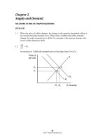
When the price of coffee changes, the change in the quantity demanded reflects a
movement along the demand curve. When other variables that affect demand
change, the entire demand curve shifts. For example, when income changes, this
causes coffee demand to shift.
∂Q
= 0.1.
∂Y

An increase in Y shifts the demand curve to the right, from D1 to D2.

97

©2017 Pearson Education, Inc.


98

1.3

Perloff/Brander, Managerial Economics and Strategy, Second Edition

The market demand curve is the sum of the quantity demanded by individual
consumers at a given price. Graphically, the market demand curve is the horizontal

sum of individual demand curves.

1.4 a. The inverse demand curve for other town residents is p = 200 – 0.5Qr.
b. At a price of $300, college students demand 100 units of firewood, and other
residents demand no firewood. Other residents will demand zero units of firewood
if the price is greater than or equal to $200.
c. The market demand curve is the horizontal sum of individual demand curves, as
illustrated below.

 

©2017 Pearson Education, Inc.


Solutions Manual—Chapter 2/Supply and Demand

99

SUPPLY
2.1

The effect of a change in pf on Q is
ΔQ
= –20pf
Δp f

ΔQ
= –20(1.10)
Δp f
ΔQ

= –22 units.
Δp f
Thus, an increase in the price of fertilizer will shift the avocado supply curve to the
left by 22 units at every price (i.e., a parallel shift to the left).
2.2

When the price of avocados changes, the change in the quantity supplied reflects a
movement along the supply curve. When costs or other variables that affect supply
change, the entire supply curve shifts. For example, the price of fertilizer represents
a key factor of avocado production, which affects the cost of avocado production,
shifting the avocado supply curve. This is because avocado prices are measured on
a graph axis. Other factors that affect supply are not measured by a graph axis.

2.3

Given the supply function,
Q = 58 + 15p – 20pf,
The effect of a change in p on Q is
ΔQ
= 15p.
Δp
To change quantity by 60, price would need to change by
60 = 15p
p = $4.00.

©2017 Pearson Education, Inc.


100

Perloff/Brander, Managerial Economics and Strategy, Second Edition

2.4

The market supply curve is the sum of the quantity supplied by individual
producers at a given price. Graphically, the market supply curve is the horizontal
sum of individual supply curves.

MARKET EQUILIBRIUM
3.1

The supply curve is upward sloping and intersects the vertical price axis at $6. The
demand curve is downward sloping and intersects the vertical price axis at $4.
When all market participants are able to buy or sell as much as they want, we say
that the market is in equilibrium: a situation in which no participant wants to change
its behavior. Graphically, a market equilibrium occurs where supply equals
demand. An equilibrium does not occur at a positive quantity because supply does
not equal demand at any price.

©2017 Pearson Education, Inc.


Solutions Manual—Chapter 2/Supply and Demand

101

3.2

The equilibrium price is p = 20 and the equilibrium quantity is Q = 80.

3.3

Given that pc = $5 and Y = $55,000 (note Y is measured in thousands, so the value
to use here is 55), the demand for coffee can be rewritten as
Q = 14 – p
and the supply of coffee can be rewritten as
Q = 8.6 + 0.5p.
When all market participants are able to buy or sell as much as they want, we say
that the market is in equilibrium: a situation in which no participant wants to change
its behavior. Graphically, a market equilibrium occurs where supply equals
demand. Thus, the equilibrium price is
D=S
14 – p = 8.6 + 0.5p
5.4 = 1.5p
p = $3.60.
Find the equilibrium quantity by substituting this price into either the supply or
demand function. For example, using the supply function, the equilibrium quantity
is
Q = 8.6 + 0.5p
Q = 8.6 + 0.5(3.60)
Q = 8.6 + 1.8
Q = 10.4 units.

©2017 Pearson Education, Inc.


102

Perloff/Brander, Managerial Economics and Strategy, Second Edition

SHOCKS TO THE EQUILIBRIUM
4.1 a. The new equilibrium with the horizontal supply curve is where the new demand
curve intersects the horizontal supply curve. The new equilibrium price is
unchanged. See figure.
b. The new equilibrium with the vertical supply curve is where the new demand
curve intersects the vertical supply curve. The new equilibrium price is higher.
See figure.
c. The new equilibrium with the upward-sloping supply curve is where the new
demand curve intersects the upward-sloping supply curve. The new equilibrium
price is higher. See figure.

©2017 Pearson Education, Inc.


Solutions Manual—Chapter 2/Supply and Demand

103

4.2 a. Health benefits from drinking coffee shift the demand curve for coffee to the right
because more coffee is now demanded at each price. The new market equilibrium
is where the original supply curve intersects the new coffee demand curve, at a
higher price and larger quantity.

b. An increase in the usefulness of cocoa will increase demand for cocoa. This
will drive up the equilibrium price of cocoa. Since cocoa and coffee are likely
substitutes, this will increase the demand for coffee. The new market
equilibrium is where the original supply curve intersects the new coffee
demand curve, at a higher price and higher quantity.

©2017 Pearson Education, Inc.

104

Perloff/Brander, Managerial Economics and Strategy, Second Edition

c. A recession shifts the demand curve for coffee to the left because less coffee
is now demanded at each price. The new market equilibrium is where the
original supply curve intersects the new coffee demand curve, at a lower price
and lower quantity.

d. New technologies increasing yields shift the supply curve for coffee to the
right because more coffee is now supplied at each price. The new market
equilibrium is where the original demand curve intersects the new coffee
supply curve, at a lower price and higher quantity.

©2017 Pearson Education, Inc.


Solutions Manual—Chapter 2/Supply and Demand

105

4.3

Outsourcing shifts the labor demand curve to the right because more Indian workers
are demanded at each wage. The new market equilibrium is where the original
supply curve intersects the new labor demand curve.

4.4

Given that pt = $0.80, the demand for avocados can be rewritten as
Q = 160 – 40p
and the supply of avocados can be rewritten as
Q = 50 + 15p.
When all market participants are able to buy or sell as much as they want, we say
that the market is in equilibrium: a situation in which no participant wants to change
its behavior. Graphically, a market equilibrium occurs where supply equals
demand. Thus, the equilibrium price is
D=S
160 – 40p = 50 + 15p
110 = 55p
p = $2.00.
Find the equilibrium quantity by substituting this price into either the supply or
demand function. For example, using the supply function, the equilibrium quantity
is
Q = 50 + 15p
Q = 50 + 15(2.00)
Q = 50 + 30
Q = 80 units.
When the price of tomatoes increases to $1.35, the demand curve for avocados
shifts out to
Q = 171 – 40p

©2017 Pearson Education, Inc.


106

Perloff/Brander, Managerial Ecconomics and Strrategy, Second E

Edition

The supply of avocadoss is unchang
ged. The new
w equilibrium
m is found w
where
D=S
171 – 40p
4 = 50 + 115p
121 = 55p
p = $2.20.
The equilib
brium quantitty is found as
a before
Q = 50 + 15p
Q = 50
5 + 15(2.200)
Q = 50 + 33
Q = 83 units.
4.5

The numbers suggest th
hat labor dem
mand is inelaastic. The suupply curve sshifts to the
right by 11 percent, yett the decrease in equilibrrium wage iss only 3.2 peercent.

4.6

o

incrreasing the eequilibrium pprice and
The damagee reduces thee supply of oranges,
decreasing the equilibriium quantity
y of orange juuice.

©2017 Pearson Educationn, Inc.


Solutions Manual—Chapter 2/Supply and Demand

107

The demand for grapefruit juice increases as the price of orange juice increases
because grapefruit juice is a substitute. As the demand for grapefruit juice increases,
the equilibrium price and quantity of grapefruit juice increase.

4.7

The increased use of corn for producing ethanol will shift the demand curve for
corn to the right. This increases the price of corn overall, reducing the consumption
of corn as food.

©2017 Pearson Education, Inc.


108

Perloff/Brander, Managerial Economics and Strategy, Second Edition

4.8

Suppose supply is initially S1, but it decreases by a small amount to S2 after the BP
oil spill. When all market participants are able to buy or sell as much as they want,
we say that the market is in equilibrium: a situation in which no participant wants to
change its behavior. Graphically, a market equilibrium occurs where supply equals
demand. The original market equilibrium is where the original demand curve
intersects the original supply curve (e1). The new market equilibrium is where the
original demand curve intersects the new supply curve (e2). When the supply curve
shifts by a relatively small amount, the change in the equilibrium price is likely to
be small.

©2017 Pearson Education, Inc.


Solutions Manual—Chapter 2/Supply and Demand

4.9

109

The Internet shifts the demand curve for newspaper advertising to the left because
fewer companies demand newspaper advertising with online advertising available.
The Internet may force some newspapers out of business, so the supply curve for
newspaper advertising will shift to the left some. The new market equilibrium is
where the new demand curve intersects the new supply curve. At the new
equilibrium, there is less newspaper advertising.

©2017 Pearson Education, Inc.

110

Perloff/Brander, Managerial Economics and Strategy, Second Edition

4.10 If global warming causes both an increase in the supply of wine during a period of
time when the demand for wine is also rising, then the overall effect on the
equilibrium quantity of wine will be for the quantity to increase. This is true
because both the increase in supply (from S1 to S2 or S3) and the increase in demand
(from D1 to D2) will result in higher equilibrium quantities on their own, and so the
combination of the two effects will definitely be an increase in quantity. The effect
of these events on the equilibrium price of wine, however, is indeterminate. The
increase in demand will lead to a higher equilibrium price, but the increase in
supply will lead to a lower equilibrium price. Taken together, the net effect on price
will be determined by how large the shifts of supply and demand are relative to one
another. If the supply shift is larger (from S1 to S2), then price will fall. If, on the
other hand, the demand shift is larger, then price will rise.

©2017 Pearson Education, Inc.


Solutions Manual—Chapter 2/Supply and Demand

111

4.11 An increase in petroleum prices shifts the aluminum supply curve to the left
because the cost of producing aluminum is more expensive at each price. An
increase in the cost of petroleum also shifts the demand curve for aluminum to the
right because the petroleum price increase makes a substitute, plastic, more
expensive (by making the cost of plastic production higher). The new equilibrium is
where the new aluminum supply curve intersects the new aluminum demand curve.

When the supply curve shifts to the left, the new equilibrium price is higher, and the
new equilibrium quantity is lower. When the demand curve shifts to the right, the
new equilibrium price is higher, and the new equilibrium quantity is higher. When
both curves shift, the new equilibrium price is higher, but the new equilibrium
quantity could be higher, lower, or unchanged.

©2017 Pearson Education, Inc.


112

Perloff/Brander, Managerial Economics and Strategy, Second Edition

4.12 The cartoon seems to show a bumper harvest of lobsters. A large increase in the
catch will shift the supply curve to the right (from S1 to S2), which will cause price
to fall from p1 to p2.

 

©2017 Pearson Education, Inc.


Solutionns Manual—Chaapter 2/Supply annd Demand

11
13

EFFE
ECTS OF GOVERNME
G

ENT INTER
RVENTION
NS
5.1

Requiring occupational
o
l licenses shiifts the laborr supply curvve to the leftt because
fewer peoplle are able to
o supply theiir labor at eaach wage. Thhe new markket
equilibrium
m is where th
he original deemand curvee intersects thhe new laboor supply
curve, at a higher
h
wage and lower employment
e
level.

5.2

In the absen
nce of price controls, thee leftward shhift of the suppply curve aas a result off
Hurricane Katrina
K
woulld push mark
ket prices upp from p0 to p1 and reducce quantity
from q0 to q1. At a goveernment imp
posed maxim
mum price off p2, consum

mers would
d
want to purrchase q uniits, but produ
ucers would only be willling to sell qs units. The
resulting sh
hortage woulld impose seearch costs on consumerss, making thhem worse
off. The red
duced quantiity and pricee also reducee firms’ profi
fits.

5.3

With a bind
ding price ceeiling, such as
a a ceiling oon the rate thhat can be chharged on
loans, somee consumers who deman
nd loans at thhe rate ceilinng will be unnable to
obtain them
m. This is beccause the dem
mand for baank loans is ggreater than the supply oof
bank loans to low-incom
me househollds with the usury law.

©2017 Pearson Educationn, Inc.


114

Perloff/Brander, Managerial Economics and Strategy, Second Edition

5.4

With the binding rent ceiling, the quantity of rental dwellings demanded is that
quantity where the rent ceiling intersects the demand curve (QD). The quantity of
rental dwellings supplied is that quantity where the rent ceiling intersects the supply
curve (QS). With the rent control laws, the quantity supplied is less than the quantity
demanded, so there is a shortage of rental dwellings.

5.5

We can determine how the total wage payment, W = wL(w), varies with respect to w
by differentiating. We then use algebra to express this result in terms of an
elasticity:
dW
dL
dL w ⎞
⎛
=L+w
= L ⎜1 +
= L (1 + ε ),
dw
dw
dw L ⎟⎠
⎝

whereε is the elasticity of demand of labor. The sign of dW/dw is the same as that of
1 + ε. Thus total labor payment decreases as the minimum wage forces up the wage
if labor demand is elastic, ε<–1, and increases if labor demand is inelastic, ε>–1.

©2017 Pearson Education, Inc.

Solutions Manual—Chapter 2/Supply and Demand

115

For a graphical explanation, see the figures below. In the top panel with very flat
supply and demand curves, the imposition of a minimum wage causes overall wage
payments to fall dramatically. On the other hand, when supply and demand curves
are steep (as in the bottom panel) overall wage payments increase substantially.

©2017 Pearson Education, Inc.


116

Perloff/Brander, Managerial Economics and Strategy, Second Edition

5.6

Before the tax is imposed, the demand for avocados can be rewritten as
Q = 160 – 40p
and the supply of avocados is given as
Q = 50 + 15p.
When all market participants are able to buy or sell as much as they want, we say
that the market is in equilibrium: a situation in which no participant wants to change
its behavior. Graphically, a market equilibrium occurs where supply equals
demand. Thus, the equilibrium price is
D=S
160 – 40p = 50 + 15p

110 = 55p
p = $2.00.
Find the equilibrium quantity by substituting this price into either the supply or
demand function. For example, using the supply function, the equilibrium quantity
is
Q = 50 + 15p
Q = 50 + 15(2.0)
Q = 50 + 30
Q = 80 units.
If a $0.55 tax is imposed, the demand curve can be rewritten to account for the tax.
First, the demand curve can be rewritten as inverse demand by solving for p
Q = 160 – 40p
p = 4 – 0.025Q.
The tax is subtracted from inverse demand to give
p = 3.45 – 0.025Q
and then this inverse demand curve can be turned back into a demand curve
Q = 138 – 40p.
Setting supply equal to demand, the new equilibrium (pretax) price is
D=S
138 – 40p = 50 + 15p
88 = 55p
p = $1.60.
The after-tax price is $2.15.

©2017 Pearson Education, Inc.


Solutions Manual—Chapter 2/Supply and Demand

117

Using the supply function, the equilibrium quantity is
Q = 50 + 15p
Q = 50 + 15(1.60)
Q = 50 + 24
Q = 74 units.
5.7

A tax on consumers will shift the demand curve down by an amount equal to the
size of the tax. The new equilibrium price and quantity with the tax will be where
the new demand curve intersects the original supply curve. The decrease in quantity
will be larger the more horizontal the supply curve is. Just the opposite, the
equilibrium quantity will not decrease at all if the supply curve is completely
vertical.

5.8 a. If demand is vertical and supply is upward sloping, then all the tax burden is paid
by consumers because they are not price sensitive.
b. If demand is horizontal and supply is upward sloping, then all the tax burden is
paid by producers because consumers are infinitely price sensitive.
c. If demand is downward sloping and supply is horizontal, then all the tax burden is
paid by consumers because producers are infinitely price sensitive.
5.9 a. A daycare subsidy shifts the demand curve for daycare up by an amount equal to
the size of the subsidy. The new equilibrium is where the new demand curve for
daycare intersects the supply curve for daycare. This is at a higher equilibrium
price and a higher equilibrium quantity.
b. See figure.

©2017 Pearson Education, Inc.

118

Perloff/Brander, Managerial Economics and Strategy, Second Edition

WHEN TO USE THE SUPPLY-AND-DEMAND MODEL
6.1

The supply-and-demand model is accurate in perfectly competitive markets, which
are markets in which all firms and consumers are price takers: no market participant
can affect the market price. If there is only one seller of a good or service—a
monopoly—that seller is a price taker and can affect the market price. Firms are
also price setters in an oligopoly—a market with only a small number of firms.
Experience has shown that the supply-and-demand model is reliable in a wide range
of markets, such as those for agriculture, financial products, labor, construction,
many services, real estate, wholesale trade, and retail trade.

MANAGERIAL PROBLEM
7.1

A tax paid by consumers shifts the demand curve down by an amount equal to the
size of the tax. Just the opposite, suspending a tax on consumers should raise the
demand curve by an amount equal to the size of the suspended tax. Although fuel
supply is more likely to be vertical in the short run than in the long run, equilibrium
fuel prices will increase when the demand curve shifts up whether the supply curve
is vertical or upward sloping.

SOLUTIONS TO SPREADSHEET EXERCISES
See the associated Excel files.

©2017 Pearson Education, Inc.

Chapter 2
Supply and Demand
CHAPTER OUTLINE
Managerial Problem: Carbon Taxes
2.1 Demand
The Demand Curve
The Demand Function
Using Calculus: Deriving the Slope of a Demand Curve
Summing Demand Curves
Mini-Case: Summing Corn Demand Curves
2.2 Supply
The Supply Curve
The Supply Function
Summing Supply Curves
2.3 Market Equilibrium
Using a Graph to Determine the Equilibrium
Using Algebra to Determine the Equilibrium
Forces That Drive the Market to Equilibrium
2.4 Shocks to the Equilibrium
Effects of a Shift in the Demand Curve
Q&A 2.1
Effects of a Shift in the Supply Curve
Managerial Implication: Taking Advantage of Future Shocks
Effects of Shifts in both Supply and Demand Curves
Mini-Case: Genetically Modified Foods
Q&A 2.2
2.5 Effects of Government Interventions
Policies That Shift Curves

Mini-Case: Occupational Licensing
Price Controls
Mini-Case: Venezuelan Price Ceilings and Shortages
Sales Taxes
Q&A 2.3
Managerial Implication: Cost Pass-Through

4

©2017 Pearson Education, Inc.


Instructor’s Manual—Chapter 2/Supply and Demand

5

2.6 When to Use the Supply-and-Demand Model
Managerial Solution: Carbon Taxes
MAIN TOPICS
1. Demand: The quantity of a good or service that consumers demand depends on
price and other factors such as consumer incomes and the prices of related goods.
2. Supply: The quantity of a good or service that firms supply depends on price and
other factors such as the cost of inputs and the level of technological sophistication
used in production.
3. Market Equilibrium: The interaction between consumers’ demand and
producers’ supply determines the market price and quantity of a good or service
that is bought and sold.
4. Shocks to the Equilibrium: Changes in a factor that affect demand (such as
consumer income) or supply (such as the price of inputs) alter the market price and
quantity sold of a good or service.

5. Effects of Government Interventions: Government policy may also affect the
equilibrium by shifting the demand curve or the supply curve, restricting price or
quantity, or using taxes to create a gap between the price consumers pay and the
price firms receive.
6. When to Use the Supply-and-Demand Model: The supply-and-demand model
applies very well to highly competitive markets, which are typically markets with
many buyers and sellers.

©2017 Pearson Education, Inc.


6

Perloff/Brander, Managerial Economics and Strategy, Second Edition

OVERVIEW
This is obviously an important chapter, and while much of this material will be
review for many students, a good, solid understanding of the basics here will pay big
dividends later.
Demand: This is a good place to begin because most students have experience
thinking about market situations from the perspective of a consumer. Whether
students have been exposed to this material previously or not, one of the trickiest
parts in this section is the distinction between a change in price and a change in any
of the other determinants of demand. The former, of course, leads to a change in
quantity demanded and a movement along the demand curve, while the latter leads
to a change in demand and a shift of the entire demand curve. It is helpful to point
out that this distinction is somewhat artificial and is driven by the fact that the
demand relationship is being represented graphically in two dimensions. Depending
on the mathematical preparation of the class, it can be very helpful to discuss the
demand relationship algebraically without worrying about drawing the diagram.

This allows for multiple right hand side variables in the demand function and no
concern about which one leads to which type of change. For some students, this can
be an eye-opening observation.
Supply: The discussion here parallels the discussion in the section on demand. The
biggest difference is that students are not as familiar with taking the perspective of a
producer, so additional discussion might be necessary to get them thinking in this
way. The same technical concern arises with a shift in the supply curve versus a
movement along the curve, but it can be handled the same way that it was in
discussing demand.
Market Equilibrium: If there is one result that students are likely to recall from past
coursework, it is the fact that the intersection of the supply and demand curves
marks the equilibrium point in the market. Despite this familiarity, however, it is
important to take the time to work through any parts of the discussion that are new
(e.g., solving for equilibrium price and quantity algebraically).
It is often easiest to remind students of why the intersection of supply and demand
is the equilibrium by considering prices that are both higher and lower. Label the
(potential) equilibrium price in the diagram and then ask students to think about
high prices (those above this proposed value) and low prices (those below this
value). It should be relatively easy for students to recall and see that at high prices,
there is a surplus where quantity supplied exceeds quantity demanded. It also
should be relatively easy for them to suggest that prices should fall in this
circumstance. Likewise, at low prices there will be a shortage as quantity demanded
exceeds quantity supplied. This disequilibrium should lead to rising prices. This

©2017 Pearson Education, Inc.