Link download solution manual for business statistics 2nd edition by donnelly

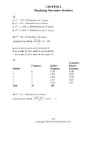
CHAPTER 2
Displaying Descriptive Statistics
2.1
a) 2 7  128  100 therefore use 7 classes.
b) 29  512  300 therefore use 9 classes.
c) 210  1, 024 1, 000 therefore use 10 classes.
d) 211  2, 048  2, 000 therefore use 11 classes.
2.2 2 6  64  50 therefore use 6 classes.
74 −16
Estimated Class Width =
= 9.7 10≈
6
a) 16-25, 26-35, 36-45, 46-55, 56-65, 66-75
b) 16 to under 26, 26 to under 36, 36 to under 46,
46 to under 56, 56 to under 66, 66 to under 76
2.3
Frequency
Number
1
2
3
4
5
Total

6
6
5
4
3
24

Relative
Frequency
0.250
0.250
0.208
0.167
0.125
1.00

2.4 25  32  30 therefore use 5 classes.
42.8 −13.9
Estimated Class Width =
= 5.8 6
5

Cumulative
Relative
Frequency
0.250
0.500
0.708
0.875
1.00

≈

2-1
Copyright ©2015 Pearson Education, Inc.

2-2 Chapter 2

Frequency
Class
13 to less than 19
19 to less than 25
25 to less than 31
31 to less than 37
37 to less than 43
Total

6
11
4
7
2
30

Relative
Frequency
0.200
0.367
0.133
0.233
0.067
1.00

Cumulative
Relative

Frequency
0.200
0.567
0.700
0.933
1.0

2.5 2 6  64  36 therefore use 6 classes.
Estimated Class Width = $5, 927 − $162 = $960 $1, 000 ≈
6
a, b, c)
Frequency
Class
Less than $1,000
$1,000 to less than $2,000
$2,000 to less than $3,000
$3,000 to less than $4,000
$4,000 to less than $5,000
$5,000 to less than $6,000
Total

12
8
3
2
6
5
36

Relative

Frequency
0.333
0.222
0.083
0.056
0.167
0.139
1.000

Cumulative
Relative
Frequency
0.333
0.555
0.638
0.694
0.861
1.000

d) The following histogram was constructed using bins $999, $1,999, $2,999, $3,999, $4,999,
and $5,999.

Copyright ©2015 Pearson Education, Inc.


Displaying Descriptive Statistics
2.6 25  32  25 therefore use 5 classes.
Estimated Class Width = 46 −18 = 5.6 6 ≈
5
a, b, c)

Frequency
Class
18-23
24-29
30-35
36-41
42-47
Total

2
6
5
5
7
25

Relative
Frequency
0.08
0.24
0.20
0.20
0.28
1.00

Cumulative
Relative
Frequency
0.08

0.32
0.52
0.72
1.00

d) The following histogram was constructed using bins 23, 29, 35, 41, and 47.

Copyright ©2015 Pearson Education, Inc.

2-3


2-4 Chapter 2
2.7
a, b, c)
Frequency
Number
0
1
2
3
4
Total

3
21
23
15
8
70

Relative
Frequency
0.043
0.300
0.329
0.214
0.114
1.000

Cumulative
Relative
Frequency
0.043
0.343
0.672
0.886
1.000

d) The following histogram was constructed using bins 0, 1, 2, 3, and 4.

2.8 2 6  64  40 therefore use 6 classes.
76 −19
Estimated Class Width (Current) =
= 9.5 10≈
6
Results would be similar using the laid-off ages.
Class
19 to less than 29
29 to less than 39

39 to less than 49
49 to less than 59
59 to less than 69
69 to less than 79

Bins
28.9
38.9
48.9
58.9
68.9
78.9

Midpoint
24
34
44
54
64
74

Copyright ©2015 Pearson Education, Inc.


Displaying Descriptive Statistics
An extra bin (18.9) was added to Excel to provide the open-ended class required by PHStat.
a)

b)

Copyright ©2015 Pearson Education, Inc.

2-5


2-6 Chapter 2
c) According to these polygons, it appears that the current workforce is younger than the laid-off
employees. It appears that the laid-off employees may have a case for age discrimination.
2.9 29  512  350 therefore use 9 classes.
$349.99 − $2.19
Estimated Class Width =
= $38.64
9
a, b, c)
Frequency
Class
Less than $40
$40 to less than $80
$80 to less than $120
$120 to less than $160
$160 to less than $200
$200 to less than $240
$240 to less than $280
$280 to less than $320
$320 to less than $360
Total

52
103
91

65
15
11
5
5
3
350

$40

≈

Relative
Frequency
0.149
0.294
0.260
0.186
0.043
0.031
0.014
0.014
0.009
1.000

Cumulative
Relative
Frequency
0.149
0.443

0.703
0.889
0.932
0.963
0.977
0.991
1.000

d) The following histogram was constructed using bins 39.999, 79.999, 119.999, 159.999,
199.999, 239.999, 279.999, 319.999, and 359.999.

Copyright ©2015 Pearson Education, Inc.


Displaying Descriptive Statistics
2.10 2 7  128  125 therefore use 7 classes.
83.2 − 71.0
Estimated Class Width =
= 1.7 2
7
a, b, c)
Frequency
Class
71 to less than 73
73 to less than 75
75 to less than 77
77 to less than 79
79 to less than 81
81 to less than 83
83 to less than 85

Total

5
37
44
31
6
1
1
125

2-7

≈

Relative
Frequency
0.040
0.296
0.352
0.248
0.048
0.008
0.008
1.000

Cumulative
Relative
Frequency
0.040

0.336
0.688
0.936
0.984
0.992
1.000

d) The following histogram was constructed using bins 72.99, 74.99, 76.99, 78.99, 80.99, 82.99,
and 84.99.

e) For 68.8% of the days, ocean temps were lower than 77 degrees.

Copyright ©2015 Pearson Education, Inc.


2-8 Chapter 2
2.11
a, b, c)
Frequency
Category
Google
Yahoo
Bing
Baidu
Other
Total

20
5
2

2
1
30

Relative
Frequency
0.667
0.167
0.067
0.067
0.033
1.000

Cumulative
Relative
Frequency
0.667
0.833
0.900
0.967
1.000

d)

2.12
a, b, c)
Frequency
Category
Excellent
Good

Fair
Poor
Total

16
31
8
5
60

Relative
Frequency
0.267
0.517
0.133
0.083
1.000

Cumulative
Relative
Frequency
0.267
0.783
0.917
1.000

Copyright ©2015 Pearson Education, Inc.


Displaying Descriptive Statistics

d)

e) 78.3% rated their dining experience as either Excellent or Good.
2.13

Copyright ©2015 Pearson Education, Inc.

2-9


2-10 Chapter 2
2.14

2.15

Copyright ©2015 Pearson Education, Inc.


Displaying Descriptive Statistics
2.16

2.17

2.18

Copyright ©2015 Pearson Education, Inc.

2-11

2-12 Chapter 2
2.19 Because all the possible categories appear to be included in the data, a pie chart would be
a good choice to display this data.

2.20 Because we are comparing data from a sample of countries over different time periods, a
clustered bar chart would be a good choice to display this data. A stacked bar chart would not be
the best choice because adding the GDPs for 2 time periods that are 10 years apart is not very
meaningful.

2.21
Grade
A
B
C
Total

Female
5
5
2
12

Male
2
7
3
12

Total
7

12
5
24

Copyright ©2015 Pearson Education, Inc.


Displaying Descriptive Statistics

2-13

71% (5/7) of the As were earned by females even though they comprise of 50% (12/24) of the
students in the class. The females appear to have done better grade-wise than the males.
2.22
Rating
1
2
3
4
Total

Darby
0
2
6
7
15

Exton
2

3
7
3
15

Media
3
8
7
2
20

Total
5
13
20
12
50

Darby received 58% (7/12) of the 4-star ratings even though they were only 30% (15/50) of the
surveyed customers. Darby appears to have higher customer satisfaction when compared to the
other two locations.
2.23
7| 1 2 3 4 5 8 8 9
8| 0 3 6 6 7 7
9| 0 0 4 7 9
10 | 0 1 7 7
11 | 0 1 1 2 5 6 8
12 | 0 0 2 5 6
13 | 0 4 4 7 9

2.24
10 | 0 2 5 8 8 9
11 | 0 1 2 3 3 4 4 5
12 | 1 1 1 2 3 3 5 6 7 7 9
13 | 0 2 2 6 7 7 7 9
14 | 0 0 2 5 6
15 | 0
2.25 a)
1|36
2|123479
3|57778
4|00123344557889
5|0011224589
6|47
Copyright ©2015 Pearson Education, Inc.


2-14 Chapter 2
b)
1 (0) | 3
1 (5) | 6
2 (0) | 1 2 3 4
2 (5) | 7 9
3 (0) |
3 (5) | 5 7 7 7 8
4 (0) | 0 0 1 2 3 3 4 4
4 (5) | 5 5 7 8 8 9
5 (0) | 0 0 1 1 2 2 4
5 (5) | 5 8 9
6 (0) | 4

6 (5) | 7
2.26 a)
2|34678
3|0012224455556779
4|2235
b)
2 (0) | 3 4
2 (5) | 6 7 8
3 (0) | 0 0 1 2 2 2 4 4
3 (5) | 5 5 5 5 6 7 7 9
4 (0) | 2 2 3
4 (5) | 5

Copyright ©2015 Pearson Education, Inc.


Displaying Descriptive Statistics
2.27 It appears that the number of Netflix subscribers is increasing during this time period.

2.28 There does not appear to be a consistent relationship between the amount of time on the
web site and the order size.

Copyright ©2015 Pearson Education, Inc.

2-15


2-16 Chapter 2
2.29

2.30 2 6  64  40 therefore use 6 classes.
Estimated Class Width = 23 − 0 = 3.8 4≈
6
a, b, c)
Frequency
Class
0-3
4-7
8-11
12-15
16-19
20-23
Total

8
5
15
3
6
3
40

Relative
Frequency
0.200
0.125
0.375
0.075
0.150
0.075

1.000

Cumulative
Relative
Frequency
0.200
0.325
0.700
0.775
0.925
1.000

d) The following histogram was constructed using bins 3, 7, 11, 15, 19, and 23.

Copyright ©2015 Pearson Education, Inc.


Displaying Descriptive Statistics

2.31
a, b, c)
Frequency

Cumulative
Relative
Frequency
0.32
0.50
0.64
0.86

0.96
1.00

Relative
Number
Frequency
0
16
0.32
1
9
0.18
2
7
0.14
3
11
0.22
4
5
0.10
5
2
0.04
Total
50
1.00
d) The following histogram was constructed using bins 0, 1, 2, 3, 4, and 5.

Copyright ©2015 Pearson Education, Inc.

2-17


2-18 Chapter 2
e) 50%
2.32 2 6  64  48 therefore use 6 classes.
1,187 − 43
Estimated Class Width =
= 190.7 200≈
6
a, b, c)
Frequency
Class
0 to under 200
200 to under 400
400 to under 600
600 to under 800
800 to under 1,000
1,000 to under 1,200
Total

15
13
11
4
4
1
48

Relative
Frequency
0.313
0.271
0.229
0.083
0.083
0.021
1.000

Cumulative
Relative
Frequency
0.313
0.584
0.813
0.896
0.979
1.000

d) The following histogram was constructed using bins 199.9, 399.9, 599.9, 799.9, 999.9,
and 1,199.9.

2.33 2 7  128  72 therefore use 7 classes.
795 −190
Estimated Class Width =
= 86.4 100≈
7

Copyright ©2015 Pearson Education, Inc.

Displaying Descriptive Statistics 2-19
a, b, c)
Frequency
Class
101-200
201-300
301-400
401-500
501-600
601-700
701-800
Total

2
2
9
15
31
9
4
72

Relative
Frequency
0.028
0.028
0.125
0.208

0.431
0.125
0.056
1.001

Cumulative
Relative
Frequency
0.028
0.056
0.181
0.389
0.820
0.945
1.001

d) The following histogram was constructed using bins 200, 300, 400, 500, 600, 700, and 800.

2.34 25  32  30 therefore use 5 classes.
100 − 66
Estimated Class Width (Day) =
= 6.8 7 ≈
5
Results would be similar using the evening grades.
Class
66-72
73-79
80-86
87-93
94-100

Bins
72
79
86
93
100

Midpoint
69
76
83
90
97

Copyright ©2015 Pearson Education, Inc.


2-20 Chapter 2
An extra bin (65) was added to Excel to provide the open-ended class required by PHStat.
a)

b)

c) The evening class grades appear to be noticeably higher than the day class grades.

Copyright ©2015 Pearson Education, Inc.


Displaying Descriptive Statistics

2.35 29  512  300 therefore use 9 classes.
Estimated Class Width =

39 −  −14
= 5.9 6
9

≈

a, b, c)
Frequency
Class
–14 to under –8
–8 to under –2
–2 to under 4
4 to under 10
10 to under 16
16 to under 22
22 to under 28
28 to under 34
34 to under 40
Total

6
28
40
58
68
61
27

9
3
300

Relative
Frequency
0.020
0.093
0.133
0.193
0.227
0.203
0.090
0.030
0.010
0.999

Relative
Cumulative
Frequency
0.020
0.113
0.246
0.439
0.666
0.869
0.959
0.989
0.999

d) The following histogram was constructed using bins –8.1, –2.1, 3.9, 9.9, 15.9, 21.9, 27.9,
33.9, and 39.9.

e) Approximately 226 out of 300 flights were not late (75.3%).

Copyright ©2015 Pearson Education, Inc.

2-21


2-22 Chapter 2
2.36 a)

b)

2.37 2 7  128  100 therefore use 7 classes.
Estimated Class Width (Wayne) = 259 −12 = 35.3 40≈
7
Results would be similar using the Dover data.
Class
1-40
41-80
81-120
121-160
161-200
201-240
241-280

Bins
40

80
120
160
200
240
280

Midpoint
20.5
60.5
100.5
140.5
180.5
220.5
260.5

An extra bin (0) was added to Excel to provide the open-ended class required by PHStat.
Copyright ©2015 Pearson Education, Inc.


Displaying Descriptive Statistics

2-23

a)

b)

c) It appears that the days on the market for homes sold in Wayne are longer than for homes sold
in Dover.

Copyright ©2015 Pearson Education, Inc.


2-24 Chapter 2
2.38 a)

b)

Copyright ©2015 Pearson Education, Inc.


Displaying Descriptive Statistics
2.39

2.40

Reason
Too long on hold
Not knowledgeable
Not courteous
Hard to understand
Too many transfers
Other
Total

Frequency
47
22
18

15
10
8
120

Relative
Frequency
0.392
0.183
0.150
0.125
0.083
0.067

Cumulative
Relative
Frequency
0.392
0.575
0.725
0.850
0.933
1.000

Copyright ©2015 Pearson Education, Inc.

2-25