Filtering and control of wireless networked systems
Bạn đang xem bản rút gọn của tài liệu. Xem và tải ngay bản đầy đủ của tài liệu tại đây (6.64 MB, 236 trang )
Studies in Systems, Decision and Control 97
Dan Zhang
Qing-Guo Wang
Li Yu
Filtering
and Control
of Wireless
Networked
Systems
www.allitebooks.com
Studies in Systems, Decision and Control
Volume 97
Series editor
Janusz Kacprzyk, Polish Academy of Sciences, Warsaw, Poland
e-mail:
www.allitebooks.com
About this Series
The series “Studies in Systems, Decision and Control” (SSDC) covers both new
developments and advances, as well as the state of the art, in the various areas of
broadly perceived systems, decision making and control- quickly, up to date and
with a high quality. The intent is to cover the theory, applications, and perspectives
on the state of the art and future developments relevant to systems, decision
making, control, complex processes and related areas, as embedded in the fields of
engineering, computer science, physics, economics, social and life sciences, as well
as the paradigms and methodologies behind them. The series contains monographs,
textbooks, lecture notes and edited volumes in systems, decision making and
control spanning the areas of Cyber-Physical Systems, Autonomous Systems,
Sensor Networks, Control Systems, Energy Systems, Automotive Systems, Biological Systems, Vehicular Networking and Connected Vehicles, Aerospace Systems, Automation, Manufacturing, Smart Grids, Nonlinear Systems, Power
Systems, Robotics, Social Systems, Economic Systems and other. Of particular
value to both the contributors and the readership are the short publication timeframe
and the world-wide distribution and exposure which enable both a wide and rapid
dissemination of research output.
More information about this series at />
www.allitebooks.com
Dan Zhang Qing-Guo Wang
Li Yu
•
Filtering and Control
of Wireless Networked
Systems
123
www.allitebooks.com
Dan Zhang
Department of Automation
Zhejiang University of Technology
Hangzhou
China
Li Yu
Department of Automation
Zhejiang University of Technology
Hangzhou
China
Qing-Guo Wang
Institute for Intelligent Systems
University of Johannesburg
Johannesburg
South Africa
ISSN 2198-4182
ISSN 2198-4190 (electronic)
Studies in Systems, Decision and Control
ISBN 978-3-319-53122-9
ISBN 978-3-319-53123-6 (eBook)
DOI 10.1007/978-3-319-53123-6
Library of Congress Control Number: 2017930955
© Springer International Publishing AG 2017
This work is subject to copyright. All rights are reserved by the Publisher, whether the whole or part
of the material is concerned, specifically the rights of translation, reprinting, reuse of illustrations,
recitation, broadcasting, reproduction on microfilms or in any other physical way, and transmission
or information storage and retrieval, electronic adaptation, computer software, or by similar or
dissimilar methodology now known or hereafter developed.
The use of general descriptive names, registered names, trademarks, service marks, etc. in this
publication does not imply, even in the absence of a specific statement, that such names are exempt
from the relevant protective laws and regulations and therefore free for general use.
The publisher, the authors and the editors are safe to assume that the advice and information in this
book are believed to be true and accurate at the date of publication. Neither the publisher nor the
authors or the editors give a warranty, express or implied, with respect to the material contained herein or
for any errors or omissions that may have been made. The publisher remains neutral with regard to
jurisdictional claims in published maps and institutional affiliations.
Printed on acid-free paper
This Springer imprint is published by Springer Nature
The registered company is Springer International Publishing AG
The registered company address is: Gewerbestrasse 11, 6330 Cham, Switzerland
www.allitebooks.com
Preface
In the last decades, the rapid developments in the communication, control and
computer technologies have had a vital impact on the control system structure. In
the traditional control systems, the connections between the sensors, controllers and
actuators are usually realized by the port to port wiring. Such a structure has certain
drawbacks such as difficult wiring and maintenance, and the low flexibility. The
drawbacks have become more severe due to the increasing size and complexity of
modern plants. A networked control system (NCS) is a control system in which the
control loops are closed through a communication network. It is gaining popularity
recently because the utilization of a multipurpose shared network to connect spatially distributed elements results in flexible architectures and it generally reduces
installation and maintenance costs. The NCSs have been successfully applied in
many practical systems such as the car automation, intelligent building, transportation networks, haptics collaboration over the Internet and unmanned aerial
vehicles.
Note that an NCS works over a network through “non-ideal channels”. This is
the main difference between the traditional control systems and NCSs. In NCSs,
phenomena such as communication delays, data dropouts, packet disorder, quantization errors and congestions may occur due to the usage of communication
channels. These imperfections would significantly degrade the system performance
and may even destabilize the control systems.
The wireless communication becomes more popular recently for its better
mobility in locations, more flexibility in system design, lower cost in implementation and greater ease in installation, compared with the wired one. While sharing
many common features and issues with the wired one as described above, the
wireless one has special issues worth mentioning. In wireless networked control
systems (WNCSs), a sensor usually has a limited power from its battery, and
replacing the battery during the operation of WSNs is very difficult. In addition,
sensor nodes are usually deployed in a wild region and they are easily affected by
the disturbances from the environment, which may cause malfunction of the sensor
nodes, e.g., the gain variations of the computational unit. However, the networked
systems should be robust or non-fragile to these disturbances.
v
vi
Preface
Due to the great challenges for the analysis and design of NCSs, especially for
wireless one, the filtering and control of such systems is an emerging research
domain of significant importance in both theory and applications. This book
addresses these challenging issues. It presents new formulations, methods and
solutions for filtering and control of wireless networked networks. It gives a timely,
comprehensive and self-contained coverage of the recent advances in a single
volume for easy access by the researchers in this domain. Special attention is paid
to the wireless one with the energy constraint and filter/controller gain variation
problems, and both centralized and distributed solutions are presented.
The book is organized as follows: Chap. 1 presents a comprehensive survey of
NCSs, which shows major research approaches to the critical issues and insights
of these problems. Chapter 2 gives the fundamentals of the system analysis, which
are often used in subsequent chapters. The first part with Chaps. 3–6 deals with
the centralized filtering of wireless networked systems, in which different approaches are presented to achieve the energy-efficient goal. The second part with
Chaps. 7–10 discusses the distributed filtering of wireless networked systems,
where the energy constraint and filter gain variation problems are addressed. The
last part with Chaps. 11–14 presents the distributed control of wireless networked
systems, where the energy constraint and controller gain variations are the main
concerns.
This book would not have been possible without supports from our colleagues.
In particular, we are indebted to Prof. Peng Shi at University of Adelaide, Australia,
and Dr. Rongyao Ling, Zhejiang University of Technology, China, for their fruitful
collaboration with us. The supports from the National Natural Science Foundation
of China under Grant 61403341, Zhejiang Provincial Natural Science Foundation
under Grant LQ14F030002, LZ15F030003 and Zhejiang Qianjiang Talent Project
under Grant Grant QJD1402018 are gratefully acknowledged.
Hangzhou, China
Johannesburg, South Africa
Hangzhou, China
August 2016
Dan Zhang
Qing-Guo Wang
Li Yu
Contents
1
Introduction . . . . . . . . . . . . . . . . . . . .
1.1 Networked Control Systems . . .
1.2 Signal Sampling . . . . . . . . . . . .
1.3 Signal Quantization. . . . . . . . . .
1.4 Communication Delay . . . . . . .
1.5 Packet Dropouts . . . . . . . . . . . .
1.6 Medium Access Constraint . . . .
1.7 Wireless Communication . . . . .
1.8 Oview of the Book . . . . . . . . . .
References . . . . . . . . . . . . . . . . . . . . . .
.
.
.
.
.
.
.
.
.
.
.
.
.
.
.
.
.
.
.
.
.
.
.
.
.
.
.
.
.
.
.
.
.
.
.
.
.
.
.
.
.
.
.
.
.
.
.
.
.
.
.
.
.
.
.
.
.
.
.
.
.
.
.
.
.
.
.
.
.
.
.
.
.
.
.
.
.
.
.
.
.
.
.
.
.
.
.
.
.
.
.
.
.
.
.
.
.
.
.
.
.
.
.
.
.
.
.
.
.
.
.
.
.
.
.
.
.
.
.
.
.
.
.
.
.
.
.
.
.
.
.
.
.
.
.
.
.
.
.
.
.
.
.
.
.
.
.
.
.
.
.
.
.
.
.
.
.
.
.
.
.
.
.
.
.
.
.
.
.
.
.
.
.
.
.
.
.
.
.
.
.
.
.
.
.
.
.
.
.
.
.
.
.
.
.
.
.
.
.
.
.
.
.
.
.
.
.
.
.
.
.
.
.
.
.
.
.
.
.
.
.
.
.
.
.
.
.
.
.
.
.
.
.
.
.
.
.
.
.
.
.
.
.
.
.
.
.
.
.
.
1
1
3
7
10
14
18
20
22
24
2
Fundamentals . . . . . . . . . . . . . . . . . .
2.1 Mathematical Preliminaries . . . .
2.2 LTI Systems . . . . . . . . . . . . . . .
2.3 Markovian Jump Systems . . . . .
2.4 Switched Systems . . . . . . . . . . .
2.5 Linear Matrix Inequalities . . . . .
References . . . . . . . . . . . . . . . . . . . . . .
.
.
.
.
.
.
.
.
.
.
.
.
.
.
.
.
.
.
.
.
.
.
.
.
.
.
.
.
.
.
.
.
.
.
.
.
.
.
.
.
.
.
.
.
.
.
.
.
.
.
.
.
.
.
.
.
.
.
.
.
.
.
.
.
.
.
.
.
.
.
.
.
.
.
.
.
.
.
.
.
.
.
.
.
.
.
.
.
.
.
.
.
.
.
.
.
.
.
.
.
.
.
.
.
.
.
.
.
.
.
.
.
.
.
.
.
.
.
.
.
.
.
.
.
.
.
.
.
.
.
.
.
.
.
.
.
.
.
.
.
.
.
.
.
.
.
.
.
.
.
.
.
.
.
.
.
.
.
.
.
.
.
.
.
.
.
.
.
.
.
.
.
.
.
.
31
31
32
35
40
44
48
3
H1 Filtering with Time-Varying Transmissions . . .
3.1 Introduction . . . . . . . . . . . . . . . . . . . . . . . . . . .
3.2 Problem Statement . . . . . . . . . . . . . . . . . . . . . .
3.3 Filter Analysis and Design . . . . . . . . . . . . . . . .
3.4 Illustrative Examples. . . . . . . . . . . . . . . . . . . . .
3.5 Conclusions . . . . . . . . . . . . . . . . . . . . . . . . . . .
References . . . . . . . . . . . . . . . . . . . . . . . . . . . . . . . . . .
.
.
.
.
.
.
.
.
.
.
.
.
.
.
.
.
.
.
.
.
.
.
.
.
.
.
.
.
.
.
.
.
.
.
.
.
.
.
.
.
.
.
.
.
.
.
.
.
.
.
.
.
.
.
.
.
.
.
.
.
.
.
.
.
.
.
.
.
.
.
.
.
.
.
.
.
.
.
.
.
.
.
.
.
.
.
.
.
.
.
.
51
51
51
56
62
66
67
4
H1 Filtering with Energy Constraint and Stochastic Gain
Variations . . . . . . . . . . . . . . . . . . . . . . . . . . . . . . . . . . . . . . . . . . . . . .
4.1 Introduction . . . . . . . . . . . . . . . . . . . . . . . . . . . . . . . . . . . . . . . .
4.2 Problem Formulation . . . . . . . . . . . . . . . . . . . . . . . . . . . . . . . . .
69
69
69
vii
viii
Contents
4.3 Filter Analysis and Design . . . .
4.4 An Illustrative Example . . . . . .
4.5 Conclusions . . . . . . . . . . . . . . .
References . . . . . . . . . . . . . . . . . . . . . .
.
.
.
.
.
.
.
.
.
.
.
.
.
.
.
.
.
.
.
.
.
.
.
.
.
.
.
.
.
.
.
.
.
.
.
.
.
.
.
.
.
.
.
.
.
.
.
.
.
.
.
.
.
.
.
.
72
78
81
81
5
H1 Filtering with Stochastic Signal Transmissions .
5.1 Introduction . . . . . . . . . . . . . . . . . . . . . . . . . . .
5.2 Problem Formulation . . . . . . . . . . . . . . . . . . . .
5.3 Filter Analysis and Design . . . . . . . . . . . . . . . .
5.4 An Illustrative Example . . . . . . . . . . . . . . . . . .
5.5 Conclusions . . . . . . . . . . . . . . . . . . . . . . . . . . .
References . . . . . . . . . . . . . . . . . . . . . . . . . . . . . . . . . .
.
.
.
.
.
.
.
.
.
.
.
.
.
.
.
.
.
.
.
.
.
.
.
.
.
.
.
.
.
.
.
.
.
.
.
.
.
.
.
.
.
.
.
.
.
.
.
.
.
.
.
.
.
.
.
.
.
.
.
.
.
.
.
.
.
.
.
.
.
.
.
.
.
.
.
.
.
.
.
.
.
.
.
.
.
.
.
.
.
.
.
83
83
83
87
91
95
96
6
H1 Filtering with Stochastic Sampling and Measurement Size
Reduction . . . . . . . . . . . . . . . . . . . . . . . . . . . . . . . . . . . . . . . . . . . . . . . 97
6.1 Introduction . . . . . . . . . . . . . . . . . . . . . . . . . . . . . . . . . . . . . . . . 97
6.2 Problem Formulation . . . . . . . . . . . . . . . . . . . . . . . . . . . . . . . . . 97
6.3 Filter Analysis and Design . . . . . . . . . . . . . . . . . . . . . . . . . . . . . 101
6.4 An Illustrative Example . . . . . . . . . . . . . . . . . . . . . . . . . . . . . . . 106
6.5 Conclusions . . . . . . . . . . . . . . . . . . . . . . . . . . . . . . . . . . . . . . . . 109
7
Distributed Filtering with Communication Reduction . .
7.1 Introduction . . . . . . . . . . . . . . . . . . . . . . . . . . . . . . .
7.2 Problem Formulation . . . . . . . . . . . . . . . . . . . . . . . .
7.3 Filter Analysis and Design . . . . . . . . . . . . . . . . . . . .
7.4 An Illustrative Example . . . . . . . . . . . . . . . . . . . . . .
7.5 Conclusions . . . . . . . . . . . . . . . . . . . . . . . . . . . . . . .
References . . . . . . . . . . . . . . . . . . . . . . . . . . . . . . . . . . . . . .
.
.
.
.
.
.
.
.
.
.
.
.
.
.
.
.
.
.
.
.
.
.
.
.
.
.
.
.
.
.
.
.
.
.
.
.
.
.
.
.
.
.
.
.
.
.
.
.
.
.
.
.
.
.
.
.
.
.
.
.
.
.
.
111
111
112
116
122
127
128
8
Distributed Filtering with Stochastic Sampling . . . .
8.1 Introduction . . . . . . . . . . . . . . . . . . . . . . . . . . .
8.2 Problem Formulation . . . . . . . . . . . . . . . . . . . .
8.3 Filter Analysis and Design . . . . . . . . . . . . . . . .
8.4 A Simulation Example . . . . . . . . . . . . . . . . . . .
8.5 Conclusions . . . . . . . . . . . . . . . . . . . . . . . . . . .
.
.
.
.
.
.
.
.
.
.
.
.
.
.
.
.
.
.
.
.
.
.
.
.
.
.
.
.
.
.
.
.
.
.
.
.
.
.
.
.
.
.
.
.
.
.
.
.
.
.
.
.
.
.
129
129
129
133
138
141
9
Distributed Filtering with Random Filter Gain Variations . . .
9.1 Introduction . . . . . . . . . . . . . . . . . . . . . . . . . . . . . . . . . . . .
9.2 Problem Formulation . . . . . . . . . . . . . . . . . . . . . . . . . . . . .
9.3 Filter Analysis and Design . . . . . . . . . . . . . . . . . . . . . . . . .
9.4 A Simulation Example . . . . . . . . . . . . . . . . . . . . . . . . . . . .
9.5 Conclusions . . . . . . . . . . . . . . . . . . . . . . . . . . . . . . . . . . . .
References . . . . . . . . . . . . . . . . . . . . . . . . . . . . . . . . . . . . . . . . . . .
.
.
.
.
.
.
.
.
.
.
.
.
.
.
.
.
.
.
.
.
.
.
.
.
.
.
.
.
143
143
144
147
151
154
154
.
.
.
.
.
.
.
.
.
.
.
.
.
.
.
.
.
.
.
.
.
.
.
.
.
.
.
.
.
.
.
.
.
.
.
.
.
.
.
.
.
.
.
.
.
.
.
.
.
.
.
.
.
.
.
.
.
.
.
.
.
.
.
.
.
.
.
.
Contents
ix
10 Distributed Filtering with Measurement Size Reduction
and Filter Gain Variations . . . . . . . . . . . . . . . . . . . . . . . .
10.1 Introduction . . . . . . . . . . . . . . . . . . . . . . . . . . . . . . .
10.2 Problem Statement . . . . . . . . . . . . . . . . . . . . . . . . . .
10.3 Filter Analysis and Design . . . . . . . . . . . . . . . . . . . .
10.4 An Illustrative Example . . . . . . . . . . . . . . . . . . . . . .
10.5 Conclusions . . . . . . . . . . . . . . . . . . . . . . . . . . . . . . .
.
.
.
.
.
.
.
.
.
.
.
.
.
.
.
.
.
.
.
.
.
.
.
.
.
.
.
.
.
.
.
.
.
.
.
.
.
.
.
.
.
.
.
.
.
.
.
.
.
.
.
.
.
.
155
155
155
159
164
168
11 Distributed Control with Controller Gain Variations . . .
11.1 Introduction . . . . . . . . . . . . . . . . . . . . . . . . . . . . . . .
11.2 Problem Formulation . . . . . . . . . . . . . . . . . . . . . . . .
11.3 Main Results. . . . . . . . . . . . . . . . . . . . . . . . . . . . . . .
11.4 An Illustrative Example . . . . . . . . . . . . . . . . . . . . . .
11.5 Conclusions . . . . . . . . . . . . . . . . . . . . . . . . . . . . . . .
References . . . . . . . . . . . . . . . . . . . . . . . . . . . . . . . . . . . . . .
.
.
.
.
.
.
.
.
.
.
.
.
.
.
.
.
.
.
.
.
.
.
.
.
.
.
.
.
.
.
.
.
.
.
.
.
.
.
.
.
.
.
.
.
.
.
.
.
.
.
.
.
.
.
.
.
.
.
.
.
.
.
.
169
169
169
172
175
179
179
12 Distributed Control with Measurement Size Reduction
and Random Fault . . . . . . . . . . . . . . . . . . . . . . . . . . . . . .
12.1 Introduction . . . . . . . . . . . . . . . . . . . . . . . . . . . . . . .
12.2 Problem Formulation . . . . . . . . . . . . . . . . . . . . . . . .
12.3 Main Results. . . . . . . . . . . . . . . . . . . . . . . . . . . . . . .
12.4 An Illustrative Example . . . . . . . . . . . . . . . . . . . . . .
12.5 Conclusions . . . . . . . . . . . . . . . . . . . . . . . . . . . . . . .
References . . . . . . . . . . . . . . . . . . . . . . . . . . . . . . . . . . . . . .
.
.
.
.
.
.
.
.
.
.
.
.
.
.
.
.
.
.
.
.
.
.
.
.
.
.
.
.
.
.
.
.
.
.
.
.
.
.
.
.
.
.
.
.
.
.
.
.
.
.
.
.
.
.
.
.
.
.
.
.
.
.
.
181
181
181
184
190
197
198
13 Distributed Control with Communication Reduction . . .
13.1 Introduction . . . . . . . . . . . . . . . . . . . . . . . . . . . . . . .
13.2 Problem Formulation . . . . . . . . . . . . . . . . . . . . . . . .
13.2.1 Sampling . . . . . . . . . . . . . . . . . . . . . . . . . . .
13.2.2 Measurement Size Reduction . . . . . . . . . . . .
13.3 Main Results. . . . . . . . . . . . . . . . . . . . . . . . . . . . . . .
13.4 An Illustrative Example . . . . . . . . . . . . . . . . . . . . . .
13.5 Conclusions . . . . . . . . . . . . . . . . . . . . . . . . . . . . . . .
.
.
.
.
.
.
.
.
.
.
.
.
.
.
.
.
.
.
.
.
.
.
.
.
.
.
.
.
.
.
.
.
.
.
.
.
.
.
.
.
.
.
.
.
.
.
.
.
.
.
.
.
.
.
.
.
.
.
.
.
.
.
.
.
.
.
.
.
.
.
.
.
199
199
199
201
202
204
209
213
14 Distributed Control with Event-Based Communication
and Topology Switching . . . . . . . . . . . . . . . . . . . . . . . . . .
14.1 Introduction . . . . . . . . . . . . . . . . . . . . . . . . . . . . . . .
14.2 Problem Formulation . . . . . . . . . . . . . . . . . . . . . . . .
14.3 Main Results. . . . . . . . . . . . . . . . . . . . . . . . . . . . . . .
14.4 A Simulation Study . . . . . . . . . . . . . . . . . . . . . . . . .
14.5 Conclusions . . . . . . . . . . . . . . . . . . . . . . . . . . . . . . .
References . . . . . . . . . . . . . . . . . . . . . . . . . . . . . . . . . . . . . .
.
.
.
.
.
.
.
.
.
.
.
.
.
.
.
.
.
.
.
.
.
.
.
.
.
.
.
.
.
.
.
.
.
.
.
.
.
.
.
.
.
.
.
.
.
.
.
.
.
.
.
.
.
.
.
.
.
.
.
.
.
.
.
215
215
216
220
226
232
232
Symbols and Notations
R
Rn
RmÂn
I
0
W [0
W>0
W\0
W60
WT
W À1
½aij
‚max ðWÞ
‚min ðWÞ
TrðWÞ
diagfÁ Á Ág
jj Á jj
sup
inf
L2 ½0; 1Þ
l2 ½0; 1Þ
Pr obfxg
Ef xg
NCS
WSN
CCL
LMI
LTI
Field of real numbers
n-dimensional real Euclidean space
Space of all m  n real matrices
Identity matrix
Zero matrix
Positive definite matrix W
Positive semi-definite matrix W
Negative definite matrix W
Negative semi-definite matrix W
Transpose of matrix W
Inverse of matrix W
A matrix composed of elements aij , i; j 2 N
Maximum eigenvalue of matrix W
Minimum eigenvalue of matrix W
Trace of matrix W
block-diagonal matrix
Euclidean norm of a vector and its induced norm of a matrix
supremum
infimum
Space of square integrable functions on ½0; 1Þ
Space of square summable infinite sequence on ½0; 1Þ
Probability of x
Expectation of x
Networked control system
Wireless sensor network
Cone complementarity linearization
Linear matrix inequality
Linear time-invariant
xi
Chapter 1
Introduction
1.1 Networked Control Systems
In the last decades, with the rapid development on the communication, control and
computer technologies, the conventional control systems have been evolving to modern networked control systems (NCSs), wherein the control loops are closed through
a communication network. The utilization of a multi-purpose shared network to
connect spatially distributed elements results in flexible architectures and generally
reduces installation and maintenance costs. Nowadays, NCSs have been extensively
applied in many practical systems such as the car automation [1], intelligent building
[2], transportation networks, haptics collaboration over the Internet [3] and unmanned
aerial vehicles [4]. A typical architecture of NCSs is shown in Fig. 1.1, and its estimation/filtering system is depicted in Fig. 1.2. In traditional control systems, each
component is connected through “ideal channels”, while, in NCSs, the connection
of each component is realized via “non-ideal channels”. This is the main difference
between the traditional control systems and NCSs.
In NCSs, the continuous-time measurement is first sampled and quantized. Then,
the measurement is transmitted to remote controller via the communication channel,
in which the signal may be delayed, lost or even sometimes not be allowed for
transmission due to the communication constraints. In recent years, the modeling,
analysis and synthesis of NCSs have received more and more attention, giving a great
number of publications in literature. Compared with the conventional point-to-point
control systems, the following new problems arise in NCSs:
• Signal sampling: an NCS is a digital control system and a continuous signal is
usually sampled at a certain time instant, and then the sampled measurement is
utilized for controller design. In the traditional digital control system, the sampling
period is usually fixed. However, in NCSs, the measurement packet may not be
transmitted when it is sampled since all the packets have to wait in a queue, and
then it is not desirable to sample the system with a fixed period.
• Signal quantization: Due to the limited communication bandwidth, the sampled signal has to be quantized and it is a common phenomenon in any digital
© Springer International Publishing AG 2017
D. Zhang et al., Filtering and Control of Wireless Networked Systems,
Studies in Systems, Decision and Control 97, DOI 10.1007/978-3-319-53123-6_1
1
2
1 Introduction
Fig. 1.1 A typical structure of NCS
Fig. 1.2 A networked estimation system
control systems. In this scenario, only a finite bit of information is available for
the controller design.
• Communication delay: The delay in NCSs includes computation delay in each
component due to the finite processing speed of devices, the waiting delay, i.e.,
the time for a packet waiting before being sent out, and the transmission delay
with which the packet goes through the communication channel. Compared with
the other two types of delays, the computational delay is usually negligible due
to the rapid development on the hardware instrument, while, the waiting delay
is determined by the transmission protocol and the impact of this delay can be
alleviated by some appropriate protocols. Hence, the transmission delay becomes
the main concern in the system analysis and design.
• Packet dropout: Due to network traffic congestions and packet transmission failures, packet dropouts are inevitable in networks, especially in a wireless network.
Actually, the propagation of long transmission delay can also be viewed as the
packet dropout phenomenon if one ignores the outdated data. In this case, the
controller or actuator has to decide what information should be used, the newest
data in the buffer or a simple zero signal.
1.1 Networked Control Systems
3
• Medium access constraint: The progress in digital computation and communication has enabled the development of distributed control systems in which multiple
sensors and actuators are connected to a centralized controller via a shared communication medium. Due to the limitations on data transmission, it is impossible
for all sensors and actuators to access to the communication channel for all the
time, leading to a new problem, the medium access constraint problem.
The network-induced problems mentioned above would certainly degrade the
control performance and may even destabilize the system [5]. In recent years, much
research effort has been devoted onto this area, and issues such as the stability analysis, state estimation, controller design and fault detection for NCSs have been widely
investigated. According to the connection nature, we can classify the NCSs into wired
and wireless communication ones. To help readers understand some basic modeling
and analysis methods for NCSs, we first discuss the NCSs with wired communication in the subsequent sections, and each for one particular network-induced issue.
Within each section, we present different approaches to the same issue. After them,
we briefly address special issues on the wireless case. This chapter will be concluded
with a short overview of the book.
1.2 Signal Sampling
An NCS is a digital control system and a continuous-time signal is usually sampled
at a certain time instant, and then the sampled measurement is utilized for controller
design. In the traditional digital control system, the sampling period is time-invariant.
However, in NCSs, the sampled measurement may not be transmitted immediately
since the sampled data has to wait in a queue, and it has been shown that the timevarying sampling period can achieve a better performance than the time-invariant
one. Some representative modeling and analysis methods for NCSs with sampleddata are discussed as follows.
Hybrid discrete/continuous approach: This approach is based on the representation of system in the form of a hybrid discrete/continuous model or more precisely,
the impulsive system, and the solution was first obtained in terms of differential
Riccati equations with jumps [6] and [7]. The hybrid system approach has been
recently applied to robust H∞ filtering with sampled-data [8]. Sampling intervalindependent LMI conditions have been derived, which were quite restrictive since
the information of sampling period was not utilized in filter design. Recently, the
impulsive system modeling of sampled-data system was also used in [9], which
introduced a new Lyapunov function with discontinuities at the impulse time. To
illustrate the main results in [9], we consider the following LTI system:
x˙ (t) = Ax(t) + Bu(t),
(1.1)
4
1 Introduction
where x and u are the state and the input of plant, respectively. Denote the sampling
time instant by tk , and let ε ≤ tk − tk−1 ≤ τMATI , where ε and τMATI are some positive
scalars. Then, using a linear state feedback controller u(t) = Kx(tk ) and defining a
T
new state ξ(t) = x T (t) zT (t) , where z(t) = x(tk ). The dynamics of system (1.1)
can be written as
˙ = Fξ(t), t = tk ,
ξ(t)
x(tk− )
, t = tk ,
ξ(tk ) =
x(tk− )
(1.2)
A Bu
and Bu = BK. Equation (1.2) means that x and z evolve accord0 0
ing to the first equation of (1.2) between tk and tk+1 , while, at tk , the value of x before
and after tk remains unchanged but the value of z is updated by x(tk− ). The stability
condition of system (1.2) was guaranteed if there exist symmetric positive definite
matrices P, R, X1 and a slack matrix N such that the following inequalities
where F =
M1 + τMATI M2 < 0,
M1 τMATI N
< 0,
∗ −τMATI R
(1.3)
(1.4)
hold, where
I
AT
P0 −
X1 I −I
BuT
−I
I
¯
−N I −I −
N T + τMATI F¯ T RF,
−I
I
¯ 1T I −I , F¯ = A Bu .
M2 =
X1 F¯ + FX
−I
M1 =
P
0
A Bu +
The above stability statement can be proved by using the Lyapunov functional
approach, and the following candidate Lyapunov function was constructed:
V = x T Px + ξ T
0
−ρ
˜ exp(Fs)ds ξ
(s + τMATI ) (F exp(Fs))T RF
+ (τMATI − ρ) (x − z)T X1 (x − z)
(1.5)
R0
and ρ = t − tk .
00
The improved impulsive system approach for NCSs with time-varying sampling
period has recently been proposed in [10], where an NCS was viewed as a interconnected hybrid system composed of an impulsive subsystem and an input delay
subsystem. A new type of time-varying discontinuous Lyapunov-Krasovskii functional was introduced to analyze the input-to-state stability (ISS) property of NCSs.
More recently, the stability of impulsive systems was studied from the hybrid system
where R˜ =
1.2 Signal Sampling
5
point of view in [11] and [12], and the convex conditions for robust stability analysis and stabilization of linear aperiodic impulsive and sampled-data systems under
dwell-time constraints have been presented.
Input delay system approach: Modeling of continuous-time systems with digital
control in the form of continuous-time systems with delayed control input was introduced by Mikheev et al. [13] and Astrom et al. [14], and further developed by Fridman
et al. [15]. In this approach, the closed-loop system became an infinite-dimensional
Delay Differential Equation (DDE) and the stability condition was obtained by using
Razumikin or Lyapunov-Krasovskii approach. The control law was represented as
the delayed control:
u(t) = ud (t) = ud (t − (t − tk )) = ud (t − τ (t)), tk ≤ t < tk + 1,
(1.6)
where τ (t) = t − tk . Then, the sampled data control system was transformed to a
time-delay system, where the time-varying delay τ (t) = t − tk is piecewise linear
with derivative 1 for t = tk . For the LTI system (1.1), the closed-loop system can be
written as
x˙ (t) = Ax(t) + Bud (t − τ (t)).
(1.7)
The recent advances on the time-delay system can be applied for the sampled data
system, e.g., the free weighting matrix approach [16] and [17], Jensen’s Inequality
approach [18] and [19], Wringter Inequality approach [20] and [21] and time-varying
Lyapunov functional approach [22]. The input delay system approach has also be
applied to the synchronization of complex networks, see [23, 24].
Robust control approach: When a time-varying sampling period is applied in
control systems, the discrete-time counterpart would become a time-varying system.
For a given continuous time system:
x˙ (t) = Ax(t) + Bu(t),
(1.8)
u(t) = Kx(tk ), ∀t ∈ [tk , tk + 1).
(1.9)
and the control input is
The discrete-time system under sampling period Tk = tk+1 − tk becomes
x(tk+1 ) = G(Tk )x(tk ),
T
(1.10)
where G(Tk ) = exp(ATk ) + 0 k exp(Ar)BdrK. It is well known that the sufficient
condition for the asymptotic stability of system (1.10) is to find a matrix P = PT > 0
such that GT (T )PG(T ) < 0 for all Tk . For a fixed sampling period T , it is easy to find
a solution of this inequality, but for any time-varying Tk with Tmin ≤ T ≤ Tmax , it is
however not easy to find the solution since infinity number of LMIs are involved. To
6
1 Introduction
conquer this problem, Suh [25] partitioned the G(k) into G(T _nom)+ΔQ(T _nom),
and T _nom is a constant to be chosen. By doing so, G(T _nom) becomes a constant matrix and the term ΔQ(T _nom) caused by the sampling interval variation was
treated as an norm bounded uncertainty, which was handled by using the robust control technique. More specifically, they partitioned G(T ) as G(Tnom ) + Δ(τ )Q(Tnom ),
τ
where Δ(τ ) = 0 exp(Ar)dr. They first show that there exists an upper bound for
Δ(τ ) such that Δ(τ ) 2 ≤ β. This bound can be obtained by solving the minimization problem:
β¯ =
min
Tmin ≤T ≤Tmax
max {β(Tmin − T ), β(Tmax − T )} .
(1.11)
Moreover, let Tnom be the sampling period corresponding to which β reaches its
minimum, then β¯ = β(Tnom ). Based on this treatment, the closed-loop system is
stable provided that there exist a symmetric positive definite matrix P and a scalar
ε > 0 such that the following inequality holds:
⎡
⎢
⎢
⎣
−P
G(Tnom )P
A B F(Tnom )
∗
−P + εI
I
P
K
0
⎤
∗
∗ ⎥
⎥<0
⎦
ε
− β¯ 2 I
(1.12)
AB
.
T
0 0 nom
To reduce the conservatism in the above condition, Suh [25] partitioned the uncertainty into N parts. But the main limitation is that the computation is high especially
when N is very large. Similar approaches have also been discussed in [26] and [27].
The research in this direction mainly focuses on how to estimate the uncertain term
to give a less conservative bound. To overcome the limitation in [25], Oishi et al.
[28] proposed three techniques, the delta-operator representation for stability analysis, the parametric uncertainty rather than the matrix uncertainty for the effect of
aperiodic sampling, and an adaptive division introduced to reduce the computation.
Specifically, they have presented an LMI based sufficient condition for all possible
parameter values and they called it as a robust LMI. In Kao et al. [29], the stability of
LTI systems with aperiodic sampling devices was tackled from a pure discrete-time
point of view, and the system was modeled as the response of a nominal discretetime LTI system in feedback interconnection with a structured uncertainty. Stability
conditions were also derived. Further improvement can also be found in [30] and
[31].
Switched system approach: The switched linear system approach was also proposed in [32] to study the sampled data control systems. To show how it works, we
consider a simple LTI system:
where F(Tnom ) = exp
x˙ (t) = Ac x(t) + Bc u(t).
(1.13)
1.2 Signal Sampling
7
It is assumed that the sampling period hk = tk+1 − tk only takes a finite number of
values. More specifically, let hk = nk T0 , where nk ∈ {i1 , · · · , iN }, i.e., 1 ≤ i1 < i2 <
· · · < iN , and T0 is termed as the basic sampling period. Then, hk takes N possible
values and hk ∈ {i1 T0 , i2 T0 , · · · , iN T0 }. The discrete-time counterpart can now be
given by
x(tk + 1) = A(hk )x(tk ) + B(hk )u(tk ),
(1.14)
where
A(hk ) = eAc hk = eAc nk T0 = eAc T0
B(hk ) =
nk T0
0
eAc r drBc =
nk −1
i=0
nk
= An0k ,
(i+1)T0
iT0
eAc r dr Bc =
nk −1
i=0
Ai0 B0 ,
with
T0
A0 = eAc T0 , B0 =
eAc r drBc .
0
One can see that A(hk ) and B(hk ) are explicitly dependent on nk , which is varying over different sampling intervals. Thus, the above discrete-time system (1.14) is
essentially a switched linear system with finite subsystems. Based on this switched
system model, the average dwell time approach from the switched system theory
was applied for the stability analysis and controller design, see [32].
In the view of the stochastic evolution of different sampling periods, the
Markovian system theory can also be applied to study the stochastic sampling problem. The modeling method is similar to the above switched system approach, but the
only difference is that the transition of different subsystems follows the Markovian
process. More specifically, Ling et al. [33] considered the distributed H∞ filtering for
NCSs with stochastic sampling, and the sampling period jumps was assumed to be
a Markovian process. Then, the well-known Markovian system theory was applied
for the stability analysis of the filtering error system. Further developments can be
found in [34]. In these results, they are assumed that the transition probabilities are
exactly known. However in some scenarios this information may not be available
[35]. Therefore, the uncertain sampling problem deserves further investigation.
1.3 Signal Quantization
Signal quantization is a common phenomenon in NCSs. The research on control with
quantized feedback is not a new topic and can be traced back to 1956 [36], in which
the effect of quantization in a sampled data system was studied. In [37], Delchamps
showed that if a linear system is open-loop unstable, there exists a minimum rate for
8
1 Introduction
the coding of the feedback information to achieve stabilization. Since then, various
methods have been proposed to study the quantized feedback control problem. The
utilization of quantizer will result in two phenomena, i.e., saturation and performance
deterioration around the original point, which may destabilize the system. Research
on quantized feedback can be categorized, depending on whether the quantizer is
static or dynamic. The logarithmic quantizer is a kind of static quantizer and the
uniform quantizer is basically a dynamical one.
Logarithmic quantization: This quantizer Q(•) is usually symmetric and timeinvariant, i.e., Q(v) = −Q(−v). The set of quantization levels is described as
U = ±κi , κi = ρi κ0 , i = 0, ±1, ±2, ...
∪ {±κ0 } ∪ {0} , 0 < ρ < 1, κ0 > 0.
(1.15)
The quantized output Q(•) is given by:
⎧
1
κi < v <
⎨ κi , if 1+δ
Q(v) = 0, if v = 0,
⎩
−Q(−v), if v < 0,
1
κ ,v
1−δ i
> 0,
(1.16)
where δ = 1−ρ
< 1, with the quantization density 0 < ρ < 1. The illustration of
1+ρ
logarithmic quantization is depicted in Fig. 1.3.
Elia et al. [38] considered quadratic stabilization problem of a discrete-time singleinput single-output (SISO) linear time-invariant systems and it is shown that a logarithmic quantize can achieve the quadratic stabilization. Following this work, Fu
and Xie [39] proposed a sector bound approach to quantized feedback control, and
κ
κ=
κ =( +δ )
κ=
( )
δ =
Fig. 1.3 Logarithmic quantizer
κ =( −δ )
−ρ
+ρ
1.3 Signal Quantization
9
presented some interesting results for multiple-input multiple-output (MIMO) linear
discrete-time systems. For a given discrete-time LTI system
x(k + 1) = Ax(k) + Bu(k),
(1.17)
with the quantized state feedback controller u(k) = KQ(x(k)), we can define the
quantization error
e(k) = x(k) − Q(x(k)) = (I + Δ(k))x(k),
(1.18)
where Δ < δI. The closed-loop system now becomes
x(k + 1) = (A + BK(I + Δ(k))x(k).
(1.19)
The robust control approach can then be applied to study the stability and stabilization of closed-loop system since it is essentially an LTI system with norm-bounded
uncertainty. Recently, a suboptimal approach for the optimization of the number of
quantization levels was proposed in [40] and the design of a corresponding quantized
dynamic output feedback controller was also given. The sector bound approach is
effective to handle the quantization problem, which enables us to incorporate other
network-induced phenomena into the quantized control systems, e.g., the packet
dropouts [41, 42], and the communication delay [43, 44].
Uniform quantization: Brokett et al. [45] proposed the uniform quantizers with
an arbitrarily shaped quantitative area. Based on these quantizers, the “zooming”
theory was used for linear and nonlinear systems, and the sufficient condition for the
asymptotical stability was given. The uniform quantizers with an arbitrarily shaped
quantitative area have the following properties:
if x
if x
2
2
≤ Mμ, then Q(x) − x 2 ≤ Δμ,
> Mμ, then Q(x) 2 > Mμ − Δμ,
(1.20)
where M is the saturation value and Δ is the sensitivity. The first property gives
the upper bound of the quantization error when the quantized measurement is not
saturated. The second one provides the approach to test whether the quantized measurement is saturated. The illustration of uniform quantization is depicted in Fig. 1.4.
The stabilization problem was discussed recently in [46] for discrete-time linear systems with multidimensional state and one-dimensional input using quantized feedbacks with a memory structure. They have shown that in order to obtain a
control strategy which yields arbitrarily small values of T / ln C, LN/ ln C should
be big enough, where C is the contraction rate, T is the time to shrink the state of
the plant from a starting set to a target set, L is the number of the controller states,
and N is the number of the possible values that the output map of the controller
can take at each time. Recently, Liberzon et al. [47] considered the input-to-state
stabilization of linear systems with quantized state measurements. They developed a
control methodology that counteracts an unknown disturbance by switching between
10
1 Introduction
Fig. 1.4 Uniform quantizer
the so-called “zooming out” and “zooming in”, that is, when the initial state to be
quantized is saturated, the “zooming out” stage is adopted to increase the sensitivity
Δ until the state gets unsaturated, while in the “zooming in” stage, the sensitivity Δ
is reduced to push the state to zero. If the initial state to be quantized is unsaturated,
the “zooming out” stage can be omitted and the “zoom-in” stage is implemented
directly.
The “zooming out” and “zooming in” strategy has been widely used in the NCS
with quantized measurement. For example, the H∞ control for NCS with communication delay and state quantization has been studied in [48] and a unified modeling was
proposed to capture the delay and quantization. More specifically, they transformed
an NCS to a LTI system with input delay, which is the approach we have discussed
before. On the other hand, the output feedback control of NCSs with communication
delay and quantization has been studied in [49].
1.4 Communication Delay
In this section, we will focus on the transmission delay problem as other delays, e.g.,
the computation delay can be reduced by using some high performance hardware.
In a traditional control system, sensor, controller and actuator usually work based
on a fixed sampling period. But in NCSs, the above nodes can work in an eventbased mode, i.e., they can work once they have received data. It should be noted that
different work modes may lead to different models, and thus different analysis and
synthesis results would be obtained.
The communication delay can be constant or time-varying. The constant delay
occurs in NCSs when we use a buffer in the controller side and the controller reads
1.4 Communication Delay
11
the data periodically. The main limitation of such a treatment leads to much design
conservatism as we have introduced man-made delay though the packet has already
arrived but it can also be used at some fixed time instant. In other word, the delay
may have been enlarged for controller design. The analysis of NCSs with constant
delay has been discussed in Zhang et al. [50], in which the stability region was
obtained for a given constant delay. On the other hand, the controller and actuator
are usually event-driven in the NCSs, which may lead to the time-varying delay
in NCSs. Different modeling results may be obtained when different delay cases
are considered, i.e., shorter or larger than one sampling period and deterministic or
stochastic. Hence, analysis and synthesis of NCSs with time-varying delay becomes
a very active research area, and many interesting approaches are proposed.
Input delay system approach: The main idea is to transform the communication
delay into the input delay and then the recent results on the delay system approaches
are applied for the stability analysis, filter and controller designs. More specifically,
Yue et al. [51] considered the following system:
x˙ (t) = [A + ΔA(t)]x(t) + [B + ΔB(t)]u(t) + Bw w(t),
z(t) = Cx(t) + Du(t).
(1.21)
When the state information is transmitted via a communication channel, which is
subject to communication delay, system (1.21) becomes
⎧
x˙ (t) = [A + ΔA(t)]x(t) + [B + ΔB(t)]u(t) + Bw w(t),
⎪
⎪
⎨
z(t) = Cx(t) + Du(t),
⎪ u(t) = Kx(ik h),
⎪
⎩
t ∈ [ik h + τk , ik+1 h + τk+1 ),
(1.22)
where τk is the time delay at the k-th sampling time instant, and h is the sampling period. Then let ik h = t − (t − ik h), and define τ (t) = t − ik h, (1.22) can be
re-written as
⎧
x˙ (t) = [A + ΔA(t)]x(t) + [B + ΔB(t)]u(t) + Bw w(t),
⎪
⎪
⎨
z(t) = Cx(t) + Du(t),
(1.23)
u(t)
= Kx(t − τ (t)),
⎪
⎪
⎩
t ∈ [ik h + τk , ik+1 h + τk+1 ).
Then, the H∞ stabilization conditions have been presented by using the time-delay
system approach. Recently, Lam et al. [52] proposed a new NCS model, which
has two additive delays. The intention of Lam et al. was to expose a new delay
model and to give a preliminary result on its stability analysis. It is worth pointing
out that the above stability conditions have left much room for improvement. The
same problem was then considered in [53] and some less conservative stability and
H∞ controller design conditions have been obtained. More recently, Gao et. al also
proposed a modified model for the NCS with time-delay, in which the H∞ filtering
and output tracking problems were investigated, respectively, see [54] and [55].
12
1 Introduction
In Xiong et al. [56], the stabilization problem of NCSs was studied by using a logical
zero-order hold (ZOH), which was assumed to be both time-driven and event-driven,
and has the logical capability of comparing the time stamps of the arrived control
input packets and choosing the newest one to control the process. Based on the packet
time sequence analysis, the overall NCS was then discretized as a linear discrete-time
system with input delay. Till now, there are still growing papers on the input delay
system approach, and the results are extended to other complex systems such as T-S
fuzzy system [57], Markovian systems [58] and singular systems [59].
Robust control approach: The sampled system is usually modeled as a discretetime system, and the network-induced delay is treated as a variation parameter of the
system. Here, we discuss the scenario where the time-varying delay is smaller than
one sampling period. Specifically, for an LTI system
x˙ (t) = Ax(t) + Bu(t),
(1.24)
assuming that 0 ≤ τm ≤ τ (k) ≤ τM ≤ h, the discrete-time system is obtained as
x(k + 1) = (Ad + Bd0 (τ (k))K)x(k) + Bd0 (τ (k))Kx(k − 1),
(1.25)
where
h−τ (k)
Ad = eAh , Bd0 (τ (k)) =
eAs ds B, Bd1 (τ (k)) =
0
h
eAs ds B.
h−τ (k)
This system can be transformed into
x(k + 1) = G(τ (k))
x(k)
,
x(k − 1)
(1.26)
where G(τ (k)) = Ad + Bd0 (τ (k))K Bd1 (τ (k))K .
Now by partitioning G(τ (k)) as a constant term and an uncertain term, the robust
control approach can be applied to estimate the bound of the latter uncertain term,
see [60, 61] for the different bounding techniques.
Switched system approach: Although the uncertain system approach is effective, complicated numerical algorithms or parameters tuning are usually required to
guarantee that the uncertain matrix is unit norm-bounded. Unlike the above robust
control approach, Zhang et al. [62] proposed a new modeling method, where the
actuator is assumed to be time-driven, and it reads the buffer periodically at a higher
frequency than the sampling frequency, i.e., T0 = T N, where T is the sampling
period, and N ≥ 2 is a large integer. Denote the time-varying delay τk , which was
assumed to be τk < T . Then, at most two control signals can be involved in the control task during one sampling period, i.e., u(k) and u(k − 1). Let the activation time
of u(k) and u(k − 1) during one sampling period be n0 (k)T0 and n1 (k)T0 , it is easy
to see that n0 (k) + n1 (k) = N. Then for a simple LTI system:
x˙ (t) = Ap x(t) + Bp u(t),
(1.27)
1.4 Communication Delay
13
we can define A = eAp T , A0 = eAp T0 , and B0 =
system is written as
T0
0
eAp r Bp dr. Then the closed-loop
x(k + 1)
= Ax(k) + ∫Tn0 (k)T0 eAp r Bp dr × u(k − 1)
n (k)T
+ 0 0 0 eAp r Bp dr×u(k)
0 (k)+n1 (k))T0 Ap r
e Bp dr × u(k − 1)
= Ax(k) + ∫(n
n0 (k)T0
n0 (k)T0 Ap r
e Bp dr×u(k)
+ 0
n (k) n1 (k)T0 Ap r
= Ax(k) + eAp T0 0
e Bp dr×u(k − 1)
0
n0 (k)T0 Ap r
+ 0
e Bp dr×u(k)
..
.
= Ax(k) +
n1 (k)−1
i=0
A0i+n0 (k) B0 u(k − 1) +
n0 (k)−1
i=0
(1.28)
Ai0 B0 u(k).
The above system becomes a switched system as it depends on the values of n0 (k) and
n1 (k). Then the average dwell time switching scheme was applied for the exponential
stability of the closed-loop system. The above modeling idea can be tracked back to
[63], where the same working mode was firstly introduced for the NCS with timevarying delay and packet dropout. A switched system modeling was also obtained
in [64] and the NCS is presented as a discrete-time switched system with arbitrary
switching. More related results on this approach are can found in [65, 66].
Stochastic system approach: When the statistical information of delay is available for system design, the stochastic system approach can be applied. To model
the random delay, the independent identically distributed case (i.i.d) and Markovian system approach have been widely used. For the i.i.d case, a delay distribution
based stability analysis and synthesis approach for NCSs with non-uniform distribution characteristics of network communication delays was firstly considered in [67],
where the delay was partitioned into multiple different time-varying delays and each
delay has a certain bound. More specifically,
u(t) = α(t)Kx(t − τ1 (t)) + (1 − α(t))Kx(t − τ2 (t)),
(1.29)
where τ1 (t) = δ(t)τ (t), τ2 (t) = (1 − δ(t))τ (t), 0 < τ1 (t) ≤ τ1 , 0 < τ2 (t) ≤ τ2 , and
δ(t) = 0 or 1. They showed that a less conservative stability condition can be obtained
when the distribution information of time delay is used. The same delay distribution
based analysis method has been extended to fuzzy systems [68] and [69]. To reduce
the conservative of the results in [67], an improved Lyapunov-Krasovskii method
was proposed in [70] and a new bounding technique is introduced to estimate the
cross-product integral terms of the Lyapunov functional.
Recently, the Markovian system approach was proposed under the assumption
that the delay is correlated and the transition of different delays obey the Markovian
process. In [71] and [72], the network-induced random delays were modeled as
Markov chains such that the closed-loop system is a jump linear system with one
14
1 Introduction
mode. More specifically, let the delay rs (k) satisfy 0 ≤ rs (k) ≤ ds < ∞. Then, the
controller becomes
u(k) = Krs (k)x(k − rs (k)).
(1.30)
By the lifting technique, we obtain the closed-loop system:
¯ rs (k)C¯ rs (k))¯x (k),
x¯ (k + 1) = (A¯ + BK
(1.31)
where
⎡
⎡ ⎤
⎤
B
0
⎢0⎥
0⎥
⎢ ⎥
⎥
⎢ ⎥
0⎥
⎥ , B¯ = ⎢ 0 ⎥ ,
⎢ .. ⎥
.. ⎥
⎣.⎦
.⎦
0
0 0 ··· I 0
A0
⎢I 0
⎢
⎢
A¯ = ⎢ 0 I
⎢ .. ..
⎣. .
···
···
···
..
.
0
0
0
..
.
Crs (k) = 0 · · · 0 I 0 · · · 0 .
The above augmented system is a Markovian jump system and rs (k) is a Markovian chain. It should be noted that the state-feedback gain was mode-independent
in [71] and [72], the state-feedback gain only depends on the delay from sensor to
controller. Later in [73], the two random delays (sensor-to-controller and controllerto-sensor) were modeled as two different Markov chains, and the closed-loop system
was described as a Markovian jump linear system with two modes characterized by
two Markov chains. There are also some newly reported results on the NCSs with
two random delays based on the Markovian system approach and the main concerns are the design of a new mode-dependent controller with more information, see
[74, 75].
1.5 Packet Dropouts
In NCSs, the packet dropout is also inevitable, especially in a wireless networked
system. In NCSs, different transmission protocols are used, i.e., user datagram protocol (UDP) and transmission control protocol (TCP). Most results on the packet
dropouts are implicitly based on the UDP, while transmission delay may occur when
the TCP protocol is applied. The research of this area is fruitful, and the main focus
is how to model the packet dropout phenomenon and then carry out the stability
and stabilization studies based on these models. In NCSs when the packet dropout
occurs, the controller can either use the zero signal or the newest signal available in
the buffer to update the control signal, which are usually called as the zero-input and
hold-input schemes. Schenato et al. [76] discussed these schemes over a lossy link.
The expressions for computing the optimal static gain for both strategies have been