Simulation of Wireless Network Systems
Bạn đang xem bản rút gọn của tài liệu. Xem và tải ngay bản đầy đủ của tài liệu tại đây (610.13 KB, 40 trang )
13
Simulation of Wireless Network
Systems
This chapter deals with simulation of wireless network systems. We introduce the basics of
discrete-event simulation as it is the simulation technique that is used for simulating wireless
networks. We then review the main characteristics of the commonly used stochastic distribu-
tions used for the simulation of wireless networks. The techniques used to generate and test
random number sequences are investigated. Then, we introduce the techniques used to
generate random variates followed by performance metrics considerations. The chapter
concludes with cases studies on the simulation of some wireless network systems.
13.1 Basics of Discrete-Event Simulation
Simulation is a general term that is used in many disciplines including performance evalua-
tion of computer and telecommunications systems. It is the process of designing a model of a
real system and conducting experiments with this model for the purpose of understanding its
behavior, or of evaluating various strategies of its operation. Others defined simulation as the
process of experimenting with a model of the system under study using computer program-
ming. It measures a model of the system rather than the system itself.
A model is a description of a system by symbolic language or theory to be seen as a system
with which the world of objects can be expressed. Thus, a model is a system interpretation or
realization of a theory that is true. Shannon defined a model as ‘the process of designing a
computerized model of a system (or a process) and conducting experiments with this model
for the purpose either of understanding the behavior of the system or of evaluating various
strategies for the operation of the system.’
Based on the above definition of a model, we can redefine simulation as the use of a model,
which may be a computer model, to conduct experiments which, by inference, convey an
understanding of the behavior of the system under study. Simulation experiments are impor-
tant aspect of any simulation study since they help to:
†
discover something unknown or test an assumption
†
find candidate solutions, and provide a mean for evaluating them.
Basically, modeling and simulation of any system involve three types of entities: (a) real
system; (b) model; and (c) simulator. These entities are to be understood in their interrelation
to one another as they are related and dependent on each other. The real system is a source of
raw data while the model is a set of instructions for data generating. The simulator is a device
for carrying out model instructions. We need to validate and verify any simulation model in
order to make sure that the assumptions, distributions, inputs, outputs, results and conclu-
sions, as well as the simulation program (simulator), are correct [1–10].
Systems in general can be classified into stochastic and deterministic types [1–3]:
†
Stochastic systems. In this case, the system contains a certain amount of randomness in its
transitions from one state to another. A stochastic system can enter more than one possible
state in response to an activity or stimulus. Clearly, a stochastic system is nondeterministic
in the sense that the next state cannot be unequivocally predicted if the present state and
the stimulus are known.
†
Deterministic systems. Here, the new state of the system is completely determined by the
previous state and by the activity or input.
Among the reasons that make simulation attractive in predicting the performance of systems
are [1–3]:
†
Simulation can foster a creative attitude for trying new ideas. Many organizations or
companies have underutilized resources, which if fully employed, can bring about
dramatic improvements in quality and productivity. Simulation can be a cost-effective
way to express, experiment with, and evaluate such proposed solutions, strategies,
schemes, or ideas.
†
Simulation can predict outcomes for possible courses of action in a speedy way.
†
Simulation can account for the effect of variances occurring in a process or a system. It is
important to note that performance computations based solely on mean values neglect the
effect of variances. This may lead to erroneous conclusions.
†
Simulation promotes total solutions.
†
Simulation brings expertise, knowledge and information together.
†
Simulation can be cost effective in terms of time.
In order to conduct a systematic and effective simulation study and analysis, the following
phases should be followed [1,4,5]. Figure 13.1 summarizes these major steps.
†
Planning. In the planning phase, the following tasks have to be defined and identified:
–
Problem formulation. If a problem statement is being developed by the analyst, it is
important that policymakers understand and agree with the formulation.
–
Resource estimation. Here, an estimate of the resources required to collect data and
analyze the system should be conducted. Resources including time, money, personnel
and equipment, must be considered. It is better to modify goals of the simulation study
at an early stage rather than to fall short due to lack of critical resources.
–
System and data analysis. This includes a thorough search in the literature of previous
approaches, methodologies and algorithms for the same problem. Many projects have
failed due to misunderstanding of the problem at hand. Also, identifying parameters,
variables, initial conditions, and performance metrics is performed at these stages.
Furthermore, the level of detail of the model must be established.
Wireless Networks342
†
Modeling phase. In this phase, the analyst constructs a system model, which is a repre-
sentation of the real system.
–
Model building. This includes abstraction of the system into a mathematical relation-
ship with the problem formulation.
–
Data acquisition. This involves identification, specification, and collection of data.
–
Model translation. Preparation and debugging of the model for computer processing.
Models in general can be of different types. Among these are: (a) descriptive models; (b)
physical models such as the ones used in aircraft and buildings; (c) mathematical models such
as Newton’s law of motion; (d) flowcharts; (e) schematics; and (f) computer pseudo code.
The major steps in model building include: (a) preliminary simulation model diagram; (b)
construction and development of flow diagrams; (c) review model diagram with team; (d)
initiation of data collection; (e) modify the top-down design, test and validate for the required
degree of granularity; (f) complete data collection; (g) iterate through steps (e) and (g) until
the final granularity has been reached; and (h) final system diagram, transformation and
verification.
In the context of this phase, it is important to point out two concepts:
†
Model scooping. This is the process of determining what process, operation, equipment,
etc., within the system should be included in the simulation model, and at what level of
detail.
†
Level of detail. This is determined based on the component’s effect on the stability of the
Simulation of Wireless Network Systems 343
Figure 13.1 Overview of the simulation methodology [1–5]
analysis. The appropriate level of detail will vary depending on the modeling and simula-
tion goals.
13.1.1 Subsystem Modeling
When the system under simulation study is very large, a subsystem modeling is performed.
All subsystem models are later linked appropriately. In order to define/identify subsystems,
there are three general schemes:
†
Flow scheme. This scheme has been used to analyze systems that are characterized by the
flow of physical or information items through the system, such as pipeline computers.
†
Functional scheme. This scheme is useful when there are no directly observable flowing
entities in the system, such as manufacturing processes that do not use assembly lines.
†
State-change scheme. This scheme is useful in systems that are characterized by a large
number of interdependent relationships and that must be examined at regular intervals in
order to detect state changes.
13.1.2 Variable and Parameter Estimation
This is usually done by collecting data over some period of time and then computing a
frequency distribution for the desired variables. Such an analysis may help the analyst to
find a well-known distribution that can represent the behavior of the system or subsystem.
13.1.3 Selection of a Programming Language/Package
Here, the analyst should decide whether to use a general-purpose programming language, a
simulation language or a simulation package. In general, using a simulation package such as
NS2 or Opnet may save money and time, however, it may not be flexible and effective to use
simulation packages as they may not contain capabilities to do the task such as modules to
simulate the protocols or features of the network under study.
13.1.4 Verification and Validation (V&V)
Verification and validation are two important tasks that should be carried out for any simula-
tion study. They are often called V&V and many simulation journals and conferences have
special sections and tracks that deal with these tasks, respectively.
Verification is the process of finding out whether the model implements the assumptions
correctly. It is basically debugging the computer program (simulator) that implements the
model. A verified computer program can in fact represent an invalid model; a valid model can
also represent an unverified simulator.
Validation, on the other hand, refers to ensuring that the assumptions used in developing
the model are reasonable in that, if correctly implemented, the model would produce results
close to these observed in real systems. The process of model validation consists of validating
assumptions, input parameters and distributions, and output values and conclusions. Valida-
tion can be performed by one of the following techniques: (a) comparing the results of the
Wireless Networks344
simulation model with results historically produced by the real system operating under the
same conditions; (b) expert intuition; (c) theoretical (analytic) results using queuing theory or
other analytic methods; (d) another simulation model; and (e) artificial intelligence and expert
systems.
13.1.5 Applications and Experimentation
After the model has been validated and verified, it can be applied to solve the problem under
investigation. Various simulation experiments should be conducted to reveal the behavior of
the system under study. Keep in mind that it is through experimentation that the analyst can
understand the system and make recommendations about the system design and optimum
operation. The extent of experiments depends on cost to estimate performance metrics, the
sensitivity of performance metrics to specific variables and the interdependencies between
control variables [1,4,5].
The implementation of simulation findings into practice is an important task that is carried
out after experimentation. Documentation is very important and should include a full record
of the entire project activity, not just a user’s guide.
The main factors that should be considered in any simulation study are: (a) Random
Number Generators (RNGs); (b) Random Variates or observations (RVs); (c) programming
errors; (d) specification errors; (e) length of simulation; (f) sensitivity to key parameters; (g)
data collection errors in simulation; (h) optimization parameter errors; (i) incorrect design;
and (j) influence of initial conditions.
The main advantages of simulation are [4,5]:
†
Flexibility. Simulation permits controlled experimentation with the system model. Some
experiments cannot be performed on the real physical system due to inconvenience, risk
and cost.
†
Speed. Using simulation allows us to find results of experiments in a speedy manner.
Simulation permits time compression of a system over an extended period of time.
†
Simulation modeling permits sensitivity analysis by manipulating input variables. It
allows us to find the parameters that influence the simulation results. It is important to
find out which simulation parameters influence performance metrics more than others as
proper selection of their operating values is essential for stable operation.
†
Simulation modeling involves programming, mathematics, queuing theory, statistics,
system engineering and science as well as technical documentation. Clearly, it is an
excellent training tool.
The main drawbacks of simulation are [4,5]:
†
It may become expensive and time-consuming especially for large simulation models.
This will consume long computer simulation time and manpower.
†
In simulation modeling, we usually make assumptions about input variables and para-
meters, and distributions, and if these assumptions are not reasonable, this may affect the
credibility of the analysis and the conclusions.
†
When simulating large networks or systems, the time to develop the simulator (simulation
program) may become long.
Simulation of Wireless Network Systems 345
†
It is usually difficult to initialize simulation model parameters properly and not doing so
may affect the credibility of the model as well as require longer simulation time.
13.2 Simulation Models
In general, simulation models can be classified in three different dimensions [3]: (a) a static
versus dynamic simulation model, where a static model is representation of a system at a
particular time, or one that may be used to represent a system in which time plays no role,
such as Monte Carlo models, and a dynamic simulation model represents a system as it
evolves over time; (b) deterministic versus stochastic models where a deterministic model
does not contain any probabilistic components while a stochastic model has at least some
random input components; (c) continuous versus discrete simulation models where a discrete-
event simulation is concerned with modeling of a system as it evolves over time by repre-
sentation in which the state variables change instantaneously at separate points in time,
usually called events. On the other hand, continuous simulation is concerned with modeling
a system by a representation in which the state variables change continuously with respect to
time.
In order to keep track with the current value of simulation time during any simulation
study, we need a mechanism to advance simulation time from one value to another. The
variable that gives the current value of simulation time is called the simulation clock. The
schemes that can be used to advance the simulation clock are [1]:
†
Next-event time advance. In this scheme, simulation clock is initialized to zero and the
times of occurrences of future events are found out. Then simulation clock is advanced to
the time of occurrence of the most imminent event in the future event list, then the state of
the system is updated accordingly. Other future events are determined in a similar manner.
This method is repeated until the stopping condition/criterion is satisfied. Figure 13.2
summarizes the next-event time advance scheme.
†
Fixed-increment time advance. Here, simulation clock is advanced in fixed increments.
After each update of the clock, a clock is made to determine if any events should have
occurred during the previous fixed interval. If some events were scheduled to have
occurred during this interval, then they are treated as if they occurred the end of the
interval and the system state is updated accordingly.
A fixed-increment time advance scheme is not used in discrete-event simulation. This is
due to the following drawbacks: (a) errors are introduced due to processing events at the
end of the interval in which they occur; and (b) it is difficult to decide which event to
process first when events that are not simultaneous in reality are treated as such in this
scheme.
The main components that are found in most discrete-event simulation models using the
next-event time advance scheme are [1–5]: (a) system state which is the collections of state
variables necessary to describe the system at a particular time; (b) simulation clock which is a
variable giving the current value of simulated time; (c) statistical counters which are the
variables used for storing statistical information about system performance; (d) an initializing
routine which is a procedure used to initialize the simulation model at time zero; (e) a timing
routine which is a procedure that determines the next event from the event list and then
Wireless Networks346
advances the simulation clock to the time when that event is to occur; (f) an event routine
which is a procedure that updates the system state when a particular type of event occurs; (g)
library routines that are a set of subprograms used to generate random observations from
probability distributions; (h) a report generator which is a procedure that computes estimates
of the desired measures of performance and produces a report when the simulation ends; and
(i) the main program which is a procedure that invokes the timing routine in order to
determine the next event and then transfers control to the corresponding event routine to
Simulation of Wireless Network Systems 347
Figure 13.2 Summary of next-event time advance scheme [1–5]
properly update the system state, checks for termination and invokes the report generator
when the conditions for terminating the simulation are satisfied.
Simulation begins at time 0 with the main program invoking the initialization routine,
where the simulation clock is initialized to zero, the system state and statistical counters are
initialized, as well as the event list. After control has been returned to the main program, it
invokes the timing routine to find out the most eminent routine. If event i is the most eminent
one, then simulation clock is advanced to the time that this event will occur and control is
returned to the main program.
The available programming languages/packages for simulating computers and network
systems are:
†
General purpose languages such as C, C11, Java, Fortran, and Visual Basic.
†
Special simulation languages such as Simscript II.5, GPSS, GASP IV, CSIM, Modsim III.
†
Special simulation packages such as Comnet III, Network II.5, OPNet, QNAP, Network
Simulation 2 (NS-2).
13.3 Common Probability Distributions Used in Simulation
The basic logic used for extracting random values from probability distribution is based on a
Cumulative Distribution Function (CDF) and a Random Number Generator (RNG). The CDF
has Y values that range from 0 to 1. RNGs produce a set of numbers which are uniformly
distributed across this interval. For every Y value there exists a unique random variate value,
X, that can be calculated.
All commercial simulation packages do not require the simulationist to write a program
to generate random variates or observations. The coding is already contained in the package
using special statements. In such a case, a model builder simply: (a) selects a probability
distribution from which he desires random variates; (b) specifies the input parameters for
the distribution; and (c) designates a random number stream to be used with the distribu-
tion.
Standard probability distributions are usually perceived in terms of the forms produced by
their Probability Density Functions (pdf). Many probability density functions have para-
meters that control their shape and scale characteristics. There are several standard contin-
uous and discrete probability distributions that are frequently used with simulation. Examples
of these are: the exponential, gamma, normal, uniform continuous and discrete, triangular,
Erlang, Poisson, binomial, Weibull, etc. Standard probability distributions are used to repre-
sent empirical data distributions. The use of one standard distribution over the other is
dependent on the empirical data that it is representing, or the type of stochastic process
that is being modeled. It is essential to understand the key characteristics and typical applica-
tions of the standard probability distributions as this helps analysts to find a representative
distribution for empirical data and for processes where no historical data are available. Next is
a brief review of the main characteristics of the most often used probability distributions for
simulation [1–4].
†
Bernoulli distribution. This is considered the simplest discrete distribution. A Bernoulli
variate can take only two values, which are denoted as failure and success, or x ¼ 0 and
Wireless Networks348
x ¼ 1, respectively. If p represents the probability of success, then q ¼ 1 2 p is the prob-
ability of failure. The experiments to generate a Bernoulli variate are called Bernoulli
trials. This distribution is used to model the probability of an outcome having a desired
class or characteristic; for example, a packet in a computer network reaches or does not
reach the destination, and a bit in a packet is affected by noise and arrives in error. The
Bernoulli distribution and its derivative can be used only if the trials are independent and
identical.
†
Discrete uniform. This distribution can be used to represent random occurrence with
several possible outcomes. A Bernoulli (1/2) and Discrete Uniform (DU) ð0; 1Þ are the
same.
†
Uniform distribution (continuous). This distribution is also called the rectangular distribu-
tion. It is considered one of the simplest distributions to use. It is commonly used if a
random variable is bounded and no further information is available. Examples include:
distance between source and destination of message on a network, and seek time on a disk.
In order to generate a continuous uniform distribution, Uða; bÞ, you need to: generate u ,
Uð0; 1Þ and return a ¼ðb 2 aÞu. The key parameters are: a ¼ lower limit and b ¼ upper
limit, where b . a. The continuous uniform distribution is used as a ‘first’ model for a
quantity that is felt to be randomly varying between two bonds a and b, but about which
little else is known.
†
Exponential distribution. This is considered the only continuous distribution with
memoryless property. It is very popular among performance evaluation analysts who
work in simulation of computer systems and networks as well as telecommunications. It
is often used to model the time interval between events that occur according to the Poisson
process.
†
Geometric distribution. This is the discrete analog of the exponential distribution and is
usually used to represent the number of failures before the first success in a sequence of
Bernoulli trials such as the number of items inspected before finding the first defective
item.
†
Poisson distribution. This is a very popular distribution in queuing, including telephone
systems. It can be used to model the number of arrivals over a given interval such as the
number of queries to a database system over a duration, t, or the number of requests to a
server in a given duration of time, t. This distribution has a special relation with the
exponential distribution.
†
Binomial distribution. This distribution can be used to represent the number of successes
in t independent Bernoulli trials with probability p of success on each trial. Examples
include the number of nodes in a multiprocessor computer system that are active (up), the
number of bits in a packet or cell that are not affected by noise or distortion, and the
number of packets that reach the destination node with no loss.
†
Negative binomial. It is used to model the number of failures in a system before reaching
the kth success such as the number of retransmissions of a message that consists of k
packets or cells and the number of error-free bytes received on a noisy channel before the k
in-error bytes.
†
Gamma distribution. Similar to the exponential distribution, this is used in queuing model-
ing of all kinds, such as modeling service times of devices in a network.
†
Weibull Distribution. In general, this distribution is used to model lifetimes of components
such as memory or microprocessor chips used in computer and telecommunications
Simulation of Wireless Network Systems 349
systems. It can also be used to model fatigue failure and ball bearing failure. It is consid-
ered the most widely used distribution to represent failure of all types. It is interesting to
point out that the exponential distribution is a special case of the Weibull distribution when
the shape parameter a is equal to 1.
†
Normal or Gaussian distribution. This is also called the bell distribution. It is used to
model errors of any type including modeling errors and instrumentation errors. Also, it has
been found that during the wearout phase, component lifetime follows a normal distribu-
tion. A normal distribution with zero mean and a standard deviation of 1 is called standard
normal distribution or a unit normal distribution. It is interesting to note that the sum of
large uniform variates has a normal distribution. This latter characteristic is used to
generate the normal variate, among other techniques such as the rejection and Polar
techniques. This distribution is very important in statistical applications due to the central
limit theorem, which states that under general assumptions, the mean of a sample of n
mutually independent random variables, that have distribution with finite mean and
variance, is normally distributed in the limit n ! 1.
†
Lognormal distribution: The log of a normal variate has a distribution called lognormal
distribution. This distribution is used to model errors that are a product of effects of a large
number of factors. The product of a large number of positive random variates tends to have
a distribution that can be approximated by lognormal.
†
Triangle distribution. As the name indicates, the pdf of this distribution is specified by
three parameters (a, b, c) that define the coordinates of the vertices of a triangle. It can be
used as a rough model in the absence of data.
†
Erlang distribution. This distribution is usually used in queuing models. It is used to model
service times in a queuing network system as well as to model the time to repair and time
between failures.
†
Beta distribution. This distribution is used when there is no data about the system under
study. Examples include the fraction of packets or cells that need to be retransmitted.
†
Chi-square distribution. This was discovered by Karl Pearson in 1900 who used the
symbol x
2
for the sum. Since then statisticians have referred to it as the chi-square
distribution. In general, it is used whenever a sum of squares of normal variables is
involved. Examples include modeling the sample variances.
†
Student’s distribution. This was derived by Gosset who was working for a winery whose
owner did not appreciate his research. In order not to let his supervisor know about his
discovery, he published his findings in a paper under the pseudonym student. He used the
symbol t to represent the variable and hence the distribution was called the ‘student’s t
distribution’. It can be used whenever a ratio of normal variate and the square root of chi-
square variable is involved and is commonly used in setting confidence intervals and in t-
tests in statistics.
†
F-Distribution. This distribution is used in hypothesis testing. It can be generated from the
ratio of two chi-square variates. Among its applications is to model the ratio of sample
variances as in the F-test for regression and analysis of variances.
†
Pareto distribution. This is also called the double-exponential distribution, the hyperbolic
distribution, and the power-law distribution. It can be used to model the amount of CPU
time consumed by an arbitrary process, the web file size on an Internet server, and the
number of data bytes in File Transfer Protocol (FTP) bursts [8].
Wireless Networks350
13.4 Random Number Generation
In order to conduct any stochastic simulation, we need pseudorandom number sequences
that are generated using pseudorandom generators. The latter are often called Random
Number Generators (RNGs). The majority of programming languages have subroutines,
objects, or functions that generate random number sequences. The main requirements of
a random number generator are: (a) numbers produced must follow the uniform distri-
bution, since truly random events follow it; (b) the sequence of generated random
numbers produced must be reproducible (replicable) as long as the same seed is used,
which permits replication of simulation runs and facilitates debugging; (c) routines used
to generate random numbers must be fast and computationally efficient; (d) the routines
should be portable to different computer platforms and preferably to different program-
ming languages; (e) numbers produced must be statistically independent; (f) ideally, the
sequence produced must be nonrepeating for any desired length, however, this is imprac-
tical as the period must be very long; (g) the technique used should not require large
memory space; and (h) the period of the generated random sequences must be suffi-
ciently long before repeating themselves
The goal of a RNG is to generate a sequence of numbers between 0 and 1 which imitates
the ideal characteristics of uniform distribution and independence as closely as possible.
There are special tests that can be used to find out whether the generation scheme has
departed from the above goal. There are RNGs that have passed all available tests, therefore
these are recommended for use.
The algorithms that can be used to generate pseudorandom numbers are [1–4]: (a) linear
congruential generators; (b) midsquare technique; (c) Tausworthe technique; (d) extended
Fibonacci technique; and (e) combined technique.
13.4.1 Linear-Congruential Generators (LCG)
This is a widely used scheme to generate random number sequences. This technique was
initially proposed by Lehmer in 1951. In this technique, successive numbers in the sequence
are generated by the recursion relation:
X
n11
¼ðaX
n
1 bÞ mod m; for n $ 0
where m is the modulus, a is the multiplier, and b is the increment. The initial value X
0
is often called the seed. If b – 0, the form is called the mixed congruential technique.
However, when b ¼ 0, the form is called the multiplicative congruential technique. It
should be stated that the values of a, b,andm drastically affect the statistical character-
istics and period of the RNG.
Moreover, the choice of m affects the characteristics of the generated sequence.
†
Multiplicative LCG with m ¼ 2
k
. This choice of m, provides an easy mode of operation.
However, such generators do not have a full period as the maximum period for multi-
plicative LCG with modulus m ¼ 2
k
is only 1/4th of the full period, that is, 2
k
2 2. This
period is achieved if the multiplier ‘a’ is of the form 8i ^ 3 and the initial seed is an odd
integer.
†
Multiplicative LCG with m – 2
k
. In order to increase the period of the generated sequence,
the modulus m is chosen to be a prime number. A proper choice of the multiplier ‘a’, can
Simulation of Wireless Network Systems 351
give us a period of ðm 2 1Þ, which is almost equal to the maximum possible length m. Note
that unlike the mixed LCG, X
n
obtained from a multiplicative LCG can never be zero if m
is prime. The values of X
n
lie between 1 and (m 2 1), and any multiplicative LCG with a
period of (m 2 1) is called a full-period generator.
13.4.2 Midsquare Method
This method was developed by John Von Neumann in 1940. The scheme relies on the
following steps: (a) start with a seed value and square it; (b) use the middle digits of this
square as the second number in the sequence; (c) this second number is then squared and the
middle digits of this square are used as the third number of the sequence; and then (d) repeat
steps (a) to (d). Although this scheme is very simple, it has important drawbacks: (a) short
repeatability periods; (b) numbers produced may not pass randomness tests; and (c) if a 0 is
generated then all other numbers generated will be 0. The latter problem may become very
serious.
13.4.3 Tausworthe Method
This technique was developed by Tausworthe in 1965. The general form is:
b
n
¼ðC
q21
b
n21
Þ XOR ðC
q22
b
n22
Þ XOR
…
XOR ðC
0
b
n2q
Þ
where c
i
and b
i
are binary variables. The Tausworthe generator uses the last q bits of a
sequence. It can easily be implemented by hardware using Linear Feedback Shift Registers
(LFSRs).
13.4.4 Extended Fibonacci Method
A Fibonacci sequence is generated by
X
n
1 X
n21
1 X
n22
A Fibonnacci series is modified in order to generate random numbers. The modification is
X
n
1 X
n21
1 X
n22
mod m
The random number sequences generated using this technique do not have good randomness
properties, especially the fact that they have serial correlation.
The seed value in general should not affect the characteristics of the random sequence
generated. However, some seed values may affect the randomness characteristics of the RNG.
In general, good random number generators should produce good characteristics regardless of
the seed value. However, some RNGs may produce shorter sequences and inadequate
randomness characteristics if their seed values are not selected carefully. Below are recom-
mended guidelines that should be followed when selecting the seed of a random number
generator [4]:
Wireless Networks352
†
Avoid using zero. Although a zero seed may be fine for mixed LCGs, it would make a
multiplicative LCG or Tausworthe generator stick at zero.
†
Do not use even values. If the generator is not a full-period generator such as multi-
plicative LCG with modulus m ¼ 2
k
, the seed should be odd. For other cases even values
are often as good as odd values. Avoid generators that have too many restrictions.
†
Never subdivide one stream. A common mistake is to use a single stream for all variables.
For example, if (r
1
; r
2
; r
3
; …) is the sequence generated using a single seed r
0
, the analyst
may for example, use r
1
to generate interarrival times, r
2
to generate service times, and so
forth. This may result in a strong correlation between the two variables.
†
Do not use overlapping streams. Each stream of random numbers that is used to generate a
specific even should have a separate seed value. If the two seeds are such that the two
streams overlap, there will be a correlation between the streams, and the resulting
sequence will not be independent. This will lead to misleading conclusions and wrong
simulation results.
†
Make sure to reuse seeds in successive replication. When a simulation experiment is
replicated several times, the random number stream need not be reinitialized, and the
seeds left over from the previous replication can continue to be used.
†
Never use random seeds. Some simulation analysts think that using random seeds, such as
the time of the day, or current date, will give them good randomness characteristics. This is
untrue as it may cause the simulation not to be reproduced. Also, multiple streams may
overlap. Random seed selection is not recommended. Moreover, using successive random
numbers obtained from the generator as seeds is also not recommended.
13.5 Testing Random Number Generators
The desirable properties of a random number sequence are uniformity, independence and
long period. In order to make sure that the random sequence generated from a RNG have
these properties, a number of tests have been established. It is important to stress that a good
RNG should pass all available tests.
The process of testing and validating pseudorandom sequences involves the comparison of
the sequence with what would be expected from the uniform distribution. The major tech-
niques for doing so are [1–4,8]: (a) the chi-square (frequency) test; (b) the Kolmogorov–
Smirnov (K-S) test; (c) the serial test; (d) the spectral test; and (e) the poker test.
A brief description of these techniques is given below:
†
Chi-square test. This test is general and can be used for any distribution. It can be used to
test random numbers that are independent and identically uniformly distributed between 0
and 1 and for testing random variate generators. The procedure can be summarized as
follows:
1. Prepare a histogram of observed data.
2. Compare observed frequencies with those obtained from the specified density function.
3. For k cells, let O
i
¼ observed frequencies, E
i
¼ expected frequencies, then D ¼
Difference ¼
P
ðO
i
2 E
i
Þ
2
=E
i
.
4. For an exact fit D should be 0.
5. D can be shown to have a chi-square distribution with (K 2 1) degrees of freedom,
Simulation of Wireless Network Systems 353
where k is the number of cells (classes or clusters). We use the significance level a for
not rejecting or the confidence level (1 2 a) for accepting.
†
Kolmogorov–Smirnov (K-S) test. This test compares an empirical distribution function with
the distribution function, F, of the hypothesized distribution. It does not require grouping/
clustering of data into cells as in the chi-square test. Moreover, the K-S test is exact for any
sample size, n, while the chi-square test is only valid in an asymptotic sense. The K-S test
compares distribution of the set of numbers to a theoretical (uniform) distribution. The unit
interval is divided into subintervals and CDF of the sequence of numbers is calculated up to
the end of each subinterval. By comparing Ks with those listed in special tables, we can
determine if observations are uniformly distributed. In this test, the numbers are normalized
and sorted in increasing order. If the sorted numbers are: X
1
; X
2
; …X
n
such that X
n21
# X
n
.
Then two factors called K1 and K2 are calculated as follows:
K1 ¼ðnÞ
0:5
max
j
n
2 X
j
K2 ¼ðnÞ
0:5
max X
j
2
j 2 1
n
where n is the number of numbers tested and j is the order of the number under test. If the
values of K2 and K1 are smaller than K
[12a,n]
listed in the K-S tables, the observations are
said to come from the specified distribution at the a level of significance.
†
Serial test. This test measures the degree of randomness between successive numbers in a
sequence. The procedure relies on generating a sequence of M consecutive sets of N
random numbers each. Then the numbers range is partitioned into K intervals. For each
group, construct an array of size (K £ K). The array is initialized by zeros. Then, the
sequence of numbers is examined from left to right, pairwise. If the left number of a pair is
in interval i, while the right number is in interval j, increment the (i,j) element by 1. After
this, the final results of M groups are compared with each other and with expected values
using the chi-square test.
†
Spectral test. This test is used to check for a flat spectrum by checking the observed
estimated cumulative spectral density function with the K-S test. Basically, it measures
the independence of adjacent sets of numbers.
†
Poker test. The poker test treats the random numbers grouped together as a poker hand.
The hands obtained are compared with what is expected using the chi-square technique.
For more detailed information on this, see Refs. [1–6,8]
13.6 Random Variate Generation
Random number generators are used to generate sequences of numbers that follow the
uniform distribution. However, in simulation we encounter other important distributions
such as exponential, Poisson, normal, gamma, Weibull, beta, etc. In general, most simulation
analysts use existing programming library routines or special routines built into simulation
languages. However, some programming languages do not have built-in procedures for all
distributions. Therefore, it is essential that the simulation analysts understand the techniques
used to generate random variates (observations). All methods to be discussed start by gener-
Wireless Networks354
ating one or more pseudorandom number sequences from the uniform distribution. Then a
transform is applied to this uniform variate to generate the nonuniform variates. The main
techniques used to generate random variates are as follows [1,4,8].
13.6.1 The Inverse Transformation Technique
This technique can be used to sample from exponential, uniform, Weibull and triangle
distributions as well as empirical distributions. Moreover, it is considered the main technique
for sampling from a wide variety of discrete distributions.
In general, this technique is useful for transforming a standard uniform deviate into any
other distribution. The density function f(x) should be integrated to find the cumulative
density function F(x), or F(x) is an empirical distribution. The scheme is based on the
observation that given any random variable x with Cumulative Distribution Function
(CDF), F(x), the variable u ¼ FðxÞ is uniformly distributed between 0 and 1. We can obtain
x by generating uniform random numbers and computing: X ¼ F
21
(U).
Example The Exponential Distribution The Probability Density Function (pdf) is given by
f ðxÞ¼
l
e
2
l
x
; x $ 0
0; x , 0
(
The Cumulative Distribution Function (CDF) is given by
FðxÞ¼
1 2 e
2
l
x
; x $ 0
0; x , 0
(
The parameter l can be interpreted as the average number of arrivals (occurrences) per unit
time. It is equal to
l
¼ 1/
b
where
b
is interpreted as the mean interarrival time. We set the
CDF ¼ U ¼ 1 2 e
2
l
x
where U is uniformly distributed between 0 and 1.
X ¼ 2
1
l
lnð1 2 UÞ
Since U and (1 2 U) are both uniformly distributed between 0 and 1, we will use U instead of
(1 2 U) in order to reduce the computational complexity. Thus,
X ¼ 2
1
l
lnU
which is the required exponential random variate. The last expression is easy to implement
using any programming language.
13.6.2 Rejection Method
This method is also called the acceptance-rejection technique. Its efficiency depends upon
being able to minimize the number of rejections. Among the distributions that can be gener-
ated using this technique are the Poisson, gamma, beta and binomial distributions with large
N. The basis for this scheme is that the probability of r being # bf(x)isbf(x) itself. That is
Prob½r # bf ðxÞ ¼ bf ðxÞ
Simulation of Wireless Network Systems 355
where r is the standard uniform number. If x is generated randomly in the interval ðc; dÞ, and x
is rejected if r . bf ðxÞ, then the accepted x’s will satisfy the density function f(x). In order to
use this scheme, f(x) has to be bounded and x valid over some range (c # x # d). The steps to
be taken are: (1) normalize the range of f(x) such that bf ðxÞ # 1, c # x # d; (2) define x as a
uniform continuous random variable x ¼ c 1 ðd 2 cÞr; (3) generate a pair of random vari-
ables ðk
1
; k
2
Þ; (4) if the pair satisfies the property k
2
# bf ðxÞ, then set the random deviate to
x ¼ c 1 ðd 2 cÞk
1
; (5) if the test in the previous step fails, return to step 3 and repeat steps 3
and 4.
13.6.3 Composition Technique
This technique is used when the required cumulative distribution function F can be expressed
as a combination of other distributions such as F
1
,F
2
,F
3
,F
4
,…. The goal is to be able to sample
from F
i
more easily than F.
FðxÞ¼
X
p
i
F
i
ðxÞ
Moreover, this technique can be used if the probability density function f(x) can be expressed
as a weighted sum of other probability density functions.
f ðxÞ¼
X
p
i
f
i
ðxÞ
In both cases, the steps used for generation are basically the same: (a) generate a positive
random integer i such that PðI ¼ iÞ¼p
i
for i ¼ 1,2,3,…, which can be implemented using the
inverse transformation scheme; (b) return X with the ith CDF F
i
(x). The composition tech-
nique can be used to generate the Laplace (double-exponential), and the right-trapezoidal
distributions.
13.6.4 Convolution Technique
In many cases, the required random variable X can be expressed as a sum of other n random
variables (Y
i
) that are independent and identically distributed (IID). In other words,
X ¼ Y
1
1 Y
2
1
…
1 Y
n
Therefore, X can be generated by simply generating n random variates Y
i
and then summing
them. It is important to point out the difference between the convolution and composition
techniques. In the convolution scheme, the random variable X itself can be expressed as a sum
of other random variables whereas in the composition scheme, the distribution function of X
is a weighted sum of other distribution functions. Clearly, there is a fundamental difference
between the two schemes.
The algorithm used here is quite intuitive. If X is the sum of two random variables Y
1
and
Y
2
, then the pdf of X can be obtained by a convolution of the pdfs of Y
1
and Y
2
. This is why this
method is called the ‘Convolution Method.’
The convolution technique can be used to generate the Erlang, binomial, Pascal (sum of m
geometric variates), and triangular (sum of two uniform variates) distributions.
Wireless Networks356