Wang d , han z sublinear algorithms for big data applications (springer briefs in computer science) 2015
Bạn đang xem bản rút gọn của tài liệu. Xem và tải ngay bản đầy đủ của tài liệu tại đây (1.92 MB, 94 trang )
SPRINGER BRIEFS IN COMPUTER SCIENCE
Dan Wang
Zhu Han
Sublinear
Algorithms
for Big Data
Applications
123
www.allitebooks.com
SpringerBriefs in Computer Science
Series Editors
Stan Zdonik
Shashi Shekhar
Jonathan Katz
Xindong Wu
Lakhmi C. Jain
David Padua
Xuemin (Sherman) Shen
Borko Furht
VS Subrahmanian
Martial Hebert
Katsushi Ikeuchi
Bruno Siciliano
Sushil Jajodia
Newton Lee
More information about this series at />
www.allitebooks.com
www.allitebooks.com
Dan Wang • Zhu Han
Sublinear Algorithms
for Big Data Applications
123
www.allitebooks.com
Dan Wang
Department of Computing
The Hong Kong Polytechnic University
Kowloon, Hong Kong, SAR
Zhu Han
Department of Engineering
University of Houston
Houston, TX, USA
ISSN 2191-5768
ISSN 2191-5776 (electronic)
SpringerBriefs in Computer Science
ISBN 978-3-319-20447-5
ISBN 978-3-319-20448-2 (eBook)
DOI 10.1007/978-3-319-20448-2
Library of Congress Control Number: 2015943617
Springer Cham Heidelberg New York Dordrecht London
© The Author(s) 2015
This work is subject to copyright. All rights are reserved by the Publisher, whether the whole or part of
the material is concerned, specifically the rights of translation, reprinting, reuse of illustrations, recitation,
broadcasting, reproduction on microfilms or in any other physical way, and transmission or information
storage and retrieval, electronic adaptation, computer software, or by similar or dissimilar methodology
now known or hereafter developed.
The use of general descriptive names, registered names, trademarks, service marks, etc. in this publication
does not imply, even in the absence of a specific statement, that such names are exempt from the relevant
protective laws and regulations and therefore free for general use.
The publisher, the authors and the editors are safe to assume that the advice and information in this book
are believed to be true and accurate at the date of publication. Neither the publisher nor the authors or
the editors give a warranty, express or implied, with respect to the material contained herein or for any
errors or omissions that may have been made.
Printed on acid-free paper
Springer International Publishing AG Switzerland is part of Springer Science+Business Media (www.
springer.com)
www.allitebooks.com
Dedicate to my family, Dan Wang
Dedicate to my family, Zhu Han
www.allitebooks.com
www.allitebooks.com
Preface
In recent years, we see a tremendously increasing amount of data. A fundamental
challenge is how these data can be processed efficiently and effectively. On one
hand, many applications are looking for solid foundations; and on the other
hand, many theories may find new meanings. In this book, we study one specific
advancement in theoretical computer science, the sublinear algorithms and how they
can be used to solve big data application problems. Sublinear algorithms, as what
the name shows, solve problems using less than linear time or space as against to
the input size, with provable theoretical bounds. Sublinear algorithms were initially
derived from approximation algorithms in the context of randomization. While the
spirit of sublinear algorithms fit for big data application, the research of sublinear
algorithms is often restricted within theoretical computer sciences. Wide application
of sublinear algorithms, especially in the form of current big data applications, is
still in its infancy. In this book, we take a step towards bridging such gap. We first
present the foundation of sublinear algorithms. This includes the key ingredients
and the common techniques for deriving the sublinear algorithm bounds. We then
present how to apply sublinear algorithms to three big data application domains,
namely, wireless sensor networks, big data processing in MapReduce, and smart
grids. We show how problems are formalized, solved, and evaluated, such that the
research results of sublinear algorithms from the theoretical computer sciences can
be linked with real-world problems.
We would like to thank Prof. Sherman Shen for his great help in publishing this
book. This book is also supported by US NSF CMMI-1434789, CNS-1443917,
ECCS-1405121, CNS-1265268, and CNS- 0953377, National Natural Science
Foundation of China (No. 61272464), and RGC/GRF PolyU 5264/13E.
Kowloon, Hong Kong
Houston, TX, USA
Dan Wang
Zhu Han
vii
www.allitebooks.com
www.allitebooks.com
Contents
1
Introduction . . . . . . . . . . . . . . . . . . . . . . . . . . . . . . . . . . . . . . . . . . . . . . . . . . . . . . . . . . . . . . . . . . .
1.1 Big Data: The New Frontier . . . . . . . . . . . . . . . . . . . . . . . . . . . . . . . . . . . . . . . . . . . . .
1.2 Sublinear Algorithms . . . . . . . . . . . . . . . . . . . . . . . . . . . . . . . . . . . . . . . . . . . . . . . . . . . .
1.3 Book Organization . . . . . . . . . . . . . . . . . . . . . . . . . . . . . . . . . . . . . . . . . . . . . . . . . . . . . . .
References . . . . . . . . . . . . . . . . . . . . . . . . . . . . . . . . . . . . . . . . . . . . . . . . . . . . . . . . . . . . . . . . . . . . . .
1
1
4
6
7
2
Basics for Sublinear Algorithms . . . . . . . . . . . . . . . . . . . . . . . . . . . . . . . . . . . . . . . . . . . .
2.1 Introduction . . . . . . . . . . . . . . . . . . . . . . . . . . . . . . . . . . . . . . . . . . . . . . . . . . . . . . . . . . . . . .
2.2 Foundations . . . . . . . . . . . . . . . . . . . . . . . . . . . . . . . . . . . . . . . . . . . . . . . . . . . . . . . . . . . . . .
2.2.1 Approximation and Randomization. . . . . . . . . . . . . . . . . . . . . . . . . . . . .
2.2.2 Inequalities and Bounds . . . . . . . . . . . . . . . . . . . . . . . . . . . . . . . . . . . . . . . . .
2.2.3 Classification of Sublinear Algorithms . . . . . . . . . . . . . . . . . . . . . . . . .
2.3 Examples . . . . . . . . . . . . . . . . . . . . . . . . . . . . . . . . . . . . . . . . . . . . . . . . . . . . . . . . . . . . . . . . .
2.3.1 Estimating the User Percentage: The Very First Example . . . . .
2.3.2 Finding Distinct Elements . . . . . . . . . . . . . . . . . . . . . . . . . . . . . . . . . . . . . . .
2.3.3 Two-Cat Problem . . . . . . . . . . . . . . . . . . . . . . . . . . . . . . . . . . . . . . . . . . . . . . . .
2.4 Summary and Discussions . . . . . . . . . . . . . . . . . . . . . . . . . . . . . . . . . . . . . . . . . . . . . . .
References . . . . . . . . . . . . . . . . . . . . . . . . . . . . . . . . . . . . . . . . . . . . . . . . . . . . . . . . . . . . . . . . . . . . . .
9
9
10
10
11
12
13
13
14
18
20
21
3
Application on Wireless Sensor Networks . . . . . . . . . . . . . . . . . . . . . . . . . . . . . . . . .
3.1 Introduction . . . . . . . . . . . . . . . . . . . . . . . . . . . . . . . . . . . . . . . . . . . . . . . . . . . . . . . . . . . . . .
3.1.1 Background and Related Work . . . . . . . . . . . . . . . . . . . . . . . . . . . . . . . . . .
3.1.2 Chapter Outline . . . . . . . . . . . . . . . . . . . . . . . . . . . . . . . . . . . . . . . . . . . . . . . . . .
3.2 System Architecture . . . . . . . . . . . . . . . . . . . . . . . . . . . . . . . . . . . . . . . . . . . . . . . . . . . . .
3.2.1 Preliminaries . . . . . . . . . . . . . . . . . . . . . . . . . . . . . . . . . . . . . . . . . . . . . . . . . . . . .
3.2.2 Network Construction . . . . . . . . . . . . . . . . . . . . . . . . . . . . . . . . . . . . . . . . . . .
3.2.3 Specifying the Structure of the Layers. . . . . . . . . . . . . . . . . . . . . . . . . .
3.2.4 Data Collection and Aggregation . . . . . . . . . . . . . . . . . . . . . . . . . . . . . . .
3.3 Evaluation of the Accuracy and the Number of Sensors Queried . . . . .
3.3.1 MAX and MIN Queries . . . . . . . . . . . . . . . . . . . . . . . . . . . . . . . . . . . . . . . . .
3.3.2 QUANTILE Queries . . . . . . . . . . . . . . . . . . . . . . . . . . . . . . . . . . . . . . . . . . . . .
23
23
24
26
26
26
26
28
28
29
29
30
ix
www.allitebooks.com
x
Contents
3.3.3 AVERAGE and SUM Queries . . . . . . . . . . . . . . . . . . . . . . . . . . . . . . . . . .
3.3.4 Effect of the Promotion Probability p. . . . . . . . . . . . . . . . . . . . . . . . . . .
3.4 Energy Consumption. . . . . . . . . . . . . . . . . . . . . . . . . . . . . . . . . . . . . . . . . . . . . . . . . . . . .
3.4.1 Overall Lifetime of the System . . . . . . . . . . . . . . . . . . . . . . . . . . . . . . . . .
3.5 Evaluation Results . . . . . . . . . . . . . . . . . . . . . . . . . . . . . . . . . . . . . . . . . . . . . . . . . . . . . . .
3.5.1 System Settings . . . . . . . . . . . . . . . . . . . . . . . . . . . . . . . . . . . . . . . . . . . . . . . . . .
3.5.2 Layers vs. Accuracy . . . . . . . . . . . . . . . . . . . . . . . . . . . . . . . . . . . . . . . . . . . . .
3.6 Practical Variations of the Architecture . . . . . . . . . . . . . . . . . . . . . . . . . . . . . . . . .
3.7 Summary and Discussions . . . . . . . . . . . . . . . . . . . . . . . . . . . . . . . . . . . . . . . . . . . . . . .
References . . . . . . . . . . . . . . . . . . . . . . . . . . . . . . . . . . . . . . . . . . . . . . . . . . . . . . . . . . . . . . . . . . . . . .
31
37
37
38
38
39
39
42
45
45
4
Application on Big Data Processing . . . . . . . . . . . . . . . . . . . . . . . . . . . . . . . . . . . . . . . .
4.1 Introduction . . . . . . . . . . . . . . . . . . . . . . . . . . . . . . . . . . . . . . . . . . . . . . . . . . . . . . . . . . . . . .
4.1.1 Big Data Processing . . . . . . . . . . . . . . . . . . . . . . . . . . . . . . . . . . . . . . . . . . . . .
4.1.2 Overview of MapReduce . . . . . . . . . . . . . . . . . . . . . . . . . . . . . . . . . . . . . . . .
4.1.3 The Data Skew Problem . . . . . . . . . . . . . . . . . . . . . . . . . . . . . . . . . . . . . . . . .
4.1.4 Chapter Outline . . . . . . . . . . . . . . . . . . . . . . . . . . . . . . . . . . . . . . . . . . . . . . . . . .
4.2 Server Load Balancing: Analysis and Problem Formulation . . . . . . . . . .
4.2.1 Background and Motivation . . . . . . . . . . . . . . . . . . . . . . . . . . . . . . . . . . . . .
4.2.2 Problem Formulation . . . . . . . . . . . . . . . . . . . . . . . . . . . . . . . . . . . . . . . . . . . .
4.2.3 Input Models . . . . . . . . . . . . . . . . . . . . . . . . . . . . . . . . . . . . . . . . . . . . . . . . . . . . .
4.3 A 2-Competitive Fully Online Algorithm. . . . . . . . . . . . . . . . . . . . . . . . . . . . . . .
4.4 A Sampling-Based Semi-online Algorithm . . . . . . . . . . . . . . . . . . . . . . . . . . . . .
4.4.1 Sample Size . . . . . . . . . . . . . . . . . . . . . . . . . . . . . . . . . . . . . . . . . . . . . . . . . . . . . .
4.4.2 Heavy Keys . . . . . . . . . . . . . . . . . . . . . . . . . . . . . . . . . . . . . . . . . . . . . . . . . . . . . .
4.4.3 A Sample-Based Algorithm . . . . . . . . . . . . . . . . . . . . . . . . . . . . . . . . . . . . .
4.5 Performance Evaluation . . . . . . . . . . . . . . . . . . . . . . . . . . . . . . . . . . . . . . . . . . . . . . . . .
4.5.1 Simulation Setup . . . . . . . . . . . . . . . . . . . . . . . . . . . . . . . . . . . . . . . . . . . . . . . . .
4.5.2 Results on Synthetic Data . . . . . . . . . . . . . . . . . . . . . . . . . . . . . . . . . . . . . . .
4.5.3 Results on Real Data. . . . . . . . . . . . . . . . . . . . . . . . . . . . . . . . . . . . . . . . . . . . .
4.6 Summary and Discussions . . . . . . . . . . . . . . . . . . . . . . . . . . . . . . . . . . . . . . . . . . . . . . .
References . . . . . . . . . . . . . . . . . . . . . . . . . . . . . . . . . . . . . . . . . . . . . . . . . . . . . . . . . . . . . . . . . . . . . .
47
47
47
48
48
49
50
50
53
53
54
55
56
57
57
59
59
59
62
65
66
5
Application on a Smart Grid . . . . . . . . . . . . . . . . . . . . . . . . . . . . . . . . . . . . . . . . . . . . . . . .
5.1 Introduction . . . . . . . . . . . . . . . . . . . . . . . . . . . . . . . . . . . . . . . . . . . . . . . . . . . . . . . . . . . . . .
5.1.1 Background and Related Work . . . . . . . . . . . . . . . . . . . . . . . . . . . . . . . . . .
5.1.2 Chapter Outline . . . . . . . . . . . . . . . . . . . . . . . . . . . . . . . . . . . . . . . . . . . . . . . . . .
5.2 Smart Meter Data Analysis . . . . . . . . . . . . . . . . . . . . . . . . . . . . . . . . . . . . . . . . . . . . . .
5.2.1 Incomplete Data Problem . . . . . . . . . . . . . . . . . . . . . . . . . . . . . . . . . . . . . . .
5.2.2 User Usage Behavior . . . . . . . . . . . . . . . . . . . . . . . . . . . . . . . . . . . . . . . . . . . .
5.3 Load Profile Classification. . . . . . . . . . . . . . . . . . . . . . . . . . . . . . . . . . . . . . . . . . . . . . .
5.3.1 Sublinear Algorithm on Testing Two Distributions . . . . . . . . . . . .
5.3.2 Sublinear Algorithm for Classifying Users . . . . . . . . . . . . . . . . . . . . .
5.4 Differentiated Services. . . . . . . . . . . . . . . . . . . . . . . . . . . . . . . . . . . . . . . . . . . . . . . . . . .
5.5 Performance Evaluation . . . . . . . . . . . . . . . . . . . . . . . . . . . . . . . . . . . . . . . . . . . . . . . . .
5.6 Summary and Discussions . . . . . . . . . . . . . . . . . . . . . . . . . . . . . . . . . . . . . . . . . . . . . . .
References . . . . . . . . . . . . . . . . . . . . . . . . . . . . . . . . . . . . . . . . . . . . . . . . . . . . . . . . . . . . . . . . . . . . . .
69
69
71
72
73
73
74
75
75
77
78
79
80
81
Contents
6
xi
Concluding Remarks . . . . . . . . . . . . . . . . . . . . . . . . . . . . . . . . . . . . . . . . . . . . . . . . . . . . . . . . 83
6.1 Summary of the Book. . . . . . . . . . . . . . . . . . . . . . . . . . . . . . . . . . . . . . . . . . . . . . . . . . . . 83
6.2 Opportunities and Challenges . . . . . . . . . . . . . . . . . . . . . . . . . . . . . . . . . . . . . . . . . . . 84
Chapter 1
Introduction
1.1 Big Data: The New Frontier
In February 2010, National Centers for Disease Control and Prevention (CDC)
identified an outbreak of flu in the mid-Atlantic regions of the United States.
However, 2 weeks earlier, Google Flu Trends [1] had already predicted such an
outbreak. By no means does Google have more expertise in the medical domain
than the CDC. However, Google was able to predict the outbreak early because
it uses big data analytics. Google establishes an association between outbreaks of
flu and user queries, e.g., on throat pain, fever, and so on. The association is then
used to predict the flu outbreak events. Intuitively, an association means that if event
A (e.g., a certain combination of queries) happens, event B (e.g., a flu outbreak) will
happen (e.g., with high probability). One important feature of such analytics is that
the association can only be established when the data is big. When the data is small,
such as a combination of a few user queries, it may not expose any connection with
a flu outbreak. Google applied millions of models to the huge number of queries
that it has. The aforementioned prediction of flue by Google is an early example of
the power of big data analytics, and the impact of which has been profound.
The number of successful big data applications is increasing. For example,
Amazon uses massive historical shipment tracking data to recommend goods to
targeted customers. Indeed such “Target Marketing” has been adopted and is being
carried out by all business sectors that have penetrated all aspects of our life.
We see personalized recommendations from the web pages we commonly visit,
from the social network applications we use daily, and from the online game
stores we frequently access. In smart cities, data on people, the environment, and
the operational components of the city are collected and analyzed (see Fig. 1.1).
More specifically, data on traffic and air quality reports are used to determine
the causes of heavy air pollution [3], and the huge amount of data on bird
migration paths are analyzed to predict H5N1 bird flu [4]. In the area of B2B,
there are startup companies (e.g., MoleMart, MolBase) that analyze huge amount
© The Author(s) 2015
D. Wang, Z. Han, Sublinear Algorithms for Big Data Applications,
SpringerBriefs in Computer Science, DOI 10.1007/978-3-319-20448-2_1
1
2
1 Introduction
Fig. 1.1 Smart City, a big
vision of the future where
people, environment, and city
operational components are in
harmony. One key to achieve
this is big data analytics,
where data of people,
environment and city
operational components are
collected and analyzed. The
data variety is diverse, the
volume is big, the collection
velocity can be high, and the
veracity may be problematic;
yet handling these
appropriately, the value can
be significant
of data on pharmaceutical, biological, and chemical related industries. Accurate
connections between buyers and vendors are established and the risk to companies
of overstocking or understocking is reduced. This has lead to cost reductions of
more than ten times compared to current B2B intermediaries.
The expectations for the future are even greater. Today, scientists, engineers,
educators, citizens, and decision-makers have unprecedented amounts and types of
data available to them. Data come from many disparate sources, including scientific
instruments, medical devices, telescopes, microscopes, and satellites; digital media
including text, video, audio, email, weblogs, twitter feeds, image collections,
click streams, and financial transactions; dynamic sensors, social, and other types
of networks; scientific simulations, models, and surveys; or from computational
analysis of observational data. Data can be temporal, spatial, or dynamic; and
structured or unstructured. Information and knowledge derived from data can
differ in representation, complexity, granularity, context, provenance, reliability,
trustworthiness, and scope. Data can also differ in the rate at which they are
generated and accessed.
On the one hand, the enriched data provide opportunities for new observations,
new associations, and new correlations to be made, which leading to added value
and new business opportunities. On the other hand, big data poses a fundamental
challenge to the efficient processing of data. Gigabytes, terabytes or even petabytes
of data need to be processed. People commonly refer to the volume, velocity, variety,
veracity and value of data as the 5-V model. Again, take the smart city as an example
(see Fig. 1.1). The big vision of the future is that the people, environment, and city
operational components of the city be in harmony. Clearly, the variety of the data
may be great, the volume of data may be big, the collection velocity of data may be
high, and the veracity of data may be problematic; yet, handled appropriately, the
value can be significant.
1.1 Big Data: The New Frontier
3
Previous studies often focused on handling complexity in terms of
computation-intensive operations. The focus has now switched to handling
complexity in terms of data-intensive operations. In this respect, studies are carried
out on every front. Notably, there are studies from the system perspective. These
studies address the handling of big data at the processor level, at the physical
machine level, at the cloud virtualization level, and so on. There are studies on data
networking for big data communications and transmissions. There are also studies
on databases to handle fast indexing, searches, and query processing. In the system
perspective, the objective is to ensure efficient data processing performance, with
trade-offs on load balancing, fairness, accuracy, outliers, reliability, heterogeneity,
service level agreement guarantees, and so on.
Nevertheless, with the aforementioned real world applications as the demand,
and the advances of the storage, system, networking and database support as the
supply, their direct marriage may still result in unacceptable performance. As an
example, smart sensing devices, cameras, and meters are now widely deployed in
urban areas. Frequent checking needs to be made of certain properties of these
sensor data. The data is often big enough that even process each piece of the data
just once can consume a great deal of time. Studies from the system perspective
usually do not provide an answer to the issue of which data should be processed (or
given higher priority in processing) and which data may be omitted (or given a lower
priority in processing). Novel algorithms, optimizations, and learning techniques are
thus urgently needed in data analytics to wisely manage the data.
From a broader perspective, data and the knowledge discovery process involve
a cycle of analyzing data, generating a hypothesis, designing and executing new
experiments, testing the hypothesis, and refining the theory. Realizing the transformative potential of big data requires many challenges in the management of
data and knowledge to be addressed, computational methods for data analysis to
be devised, and many aspects of data-enabled discovery processes to be automated.
Combinations of computational, mathematical, and statistical techniques, methodologies and theories are needed to enable these advances to be made. There have
been many new advances in theories and methodologies on data analytics, such as
sparse optimization, tensor optimization, deep neural networks (DNN), and so on. In
applying these theories and methodologies to the applications, specific application
requirements can be taken into consideration, thus wisely reducing, shaping, and
organizing the data. Therefore, the final processing of data in the system can be
significantly more efficient than if the application data had been processed using a
brute force approach.
An overall picture of the big data processing is given in Fig. 1.2. At the top are
real world applications, where specific applications are designed and the data are
collected. Appropriated algorithms, theories, or methodologies are then applied to
assist knowledge discovery or data management. Finally, the data are stored and
processed in the execution systems, such as Hadoop, Spark, and others.
In this book, we specifically study one big data analytic theory, the sublinear
algorithm, and its use in real-world big data applications. As the name suggested, the
4
1 Introduction
Real World Applications
Smart City
Personalized
Recommendation
Precision
Marketing
...
Big Data Analytics
Sublinear
Algorithm
Tensor
DNN
...
ExecutionSystems
Hadoop
Spark
Amazon EMR
(Hadoop in Cloud)
...
Fig. 1.2 A overall picture: from real world applications to big data analytics to execution systems
performance of the sublinear algorithms, in terms of time, storage space, and so on,
is less than linear as against the amount of input data. More importantly, sublinear
algorithms provide guarantees of accuracy of the output from the algorithms.
1.2 Sublinear Algorithms
Research on sublinear algorithms began some time ago. Sublinear algorithms were
initially developed in the theoretical computer science community. The sublinear
algorithm is one further classification of the approximation algorithm. Its study
involves the long-debated issue of the trade-off between algorithm processing time
and algorithm output quality.
In a conventional approximation algorithm, the algorithm can output an approximate result that deviates from the optimal result (within a bound), yet the algorithm
processing time can become faster. One hidden implication of the design is that the
approximate result is 100 % guaranteed within this bound. In a sublinear algorithm,
such an implication is relaxed. More specifically, a sublinear algorithm outputs an
approximate result that deviates from the optimal result (within a bound) for a
(usually) majority of the time. As a concrete example, a sublinear algorithm usually
says that the output of the algorithm differs from the optimal solution by at most 0.1
(the bound) at least 95 % of the time (the confidence).
This transition is important. From the theoretical research point of view, a
new category is developed. From the practical point of view, sublinear algorithms
provide two controlling parameters for the user in making trade-offs, while approximation algorithms have only one controlling parameter.
As can be imagined, sublinear algorithms are developed based on random and
probabilistic techniques. Note, however, that the guarantee of a sublinear algorithm
is on the individual outputs of this algorithm. In this, the sublinear algorithm differs
1.2 Sublinear Algorithms
5
from stochastic techniques, which analyze the mean and variance of a system in a
steady state. For example, a typical queuing theory result is that the expected waiting
time is 100 s.
In the theoretical computer sciences in the past few years, there have been many
studies on sublinear algorithms. Sublinear algorithms have been developed for many
classic computer science problems, such as finding the most frequently element,
finding distinct elements, etc.; and for graph problems, such as finding the minimum
spanning tree, etc.; and for geometry problems, such as finding the intersection of
two polygons, etc. Sublinear algorithms can be broadly classified into sublinear time
algorithms, sublinear space algorithms, and sublinear communication algorithms,
where the amount of time, storage space, or communications needed is o.N/ with N
as the input size.
Sublinear algorithms are a good match of big data analytics. Decisions can be
drawn by only looking at a subset of the data. In particular, sublinear algorithms
are suitable for situations, where the total amount of data is so massive that even
linear processing time is not affordable. Sublinear algorithms are also suitable for
situations, where some initial investigations need to be made before looking into the
full data set. In many situations, the data are massive but it is not known whether
the value of the data is big or not. As such, sublinear algorithms can serve to give
an initial “peek” of the data before more a in-depth analysis is carried out. For
example, in bioinformatics, we need to test whether certain DNA sequences are
periodic. Sublinear algorithms, when appropriately designed to test periodicity in
data sequences, can be applied to rule out useless data.
While there have been decent advances in the past few years in research on
sublinear algorithms, to date, the study of sublinear algorithms has often been
restricted to the theoretical computer sciences. There have been some applications.
For example, in databases, where sublinear algorithms are used for the efficient
query processing such as top-k queries; in bioinformatics, sublinear algorithms are
used for testing whether a DNA sequence shows periodicity; and in networking,
sublinear algorithms are used for testing whether two network traffic flows are close
in distribution. Nevertheless, sublinear algorithms have yet to be applied, especially
in the form of current big data applications. Tutorials on sublinear algorithms from
the theoretical point of view, with a collection of different sublinear algorithms,
aimed at better approximation bounds, are particularly abundant [2]. Yet there are
far fewer applications of sublinear algorithms, aimed at application background
scenarios, problem formulations, and evaluations of parameters. This book is not a
collection of sublinear algorithms; rather, the focus is on the application of sublinear
algorithms.
In this book, we start from the foundations of the sublinear algorithm. We
discuss approximation and randomization, the later being the key to transforming a
conventional algorithm to a sublinear one. We progressively present a few examples,
showing the key ingredients of sublinear algorithms. We then discuss how to
apply sublinear algorithms in three state-of-the-art big data domains, namely, data
collection in wireless sensor networks, big data processing using MapReduce, and
6
1 Introduction
behavior analysis using metering data from smart grids. We show how the problem
should be formalized, solved, and evaluated, so that the sublinear algorithms can be
used to help solve real-world problems.
1.3 Book Organization
The purpose of this book is to give a snapshot of sublinear algorithms and their
applications. Different from other writings on sublinear algorithms, we focus
on learning the basic ideas of sublinear algorithms, rather than on presenting a
comprehensive survey of the sublinear algorithms found in literature. We also target
the issue of when and how to apply sublinear algorithms to applications. This
includes learning in what situations the sublinear algorithms may fit into certain
scenarios, how we may combine multiple sublinear algorithms to solve a problem,
how to develop sublinear algorithms with additional statistical information, what
structures are needed to support sublinear algorithms, and how we may extend
existing sublinear algorithms to fit into applications. The remaining five chapters
of the book are organized as follows.
In Chap. 2, we present the basic concepts of the sublinear algorithm. We
first present the main thread of theoretical research on sublinear algorithms and
discuss how sublinear algorithms are related to other theoretical developments in
the computing sciences, in particular, approximation and randomization. We then
present preliminary mathematical techniques on inequalities and bounds. We then
give three examples. The first is on estimating the percentage of households among
a group of people. This is an illustration of the direct application of inequalities and
bounds to derive a sublinear algorithm. The second is on finding distinct elements.
This is a classical sublinear algorithm. The example involves some key insights
and techniques in the development of sublinear algorithms. The third is a two cat
problem where we develop an algorithm that is sublinear, but which does not fall
into standard sublinear algorithm format. The example provides some additional
thoughts on the wide spectrum of sublinear algorithms.
In Chap. 3, we present an application of sublinear algorithms in wireless sensor
data collection. Data collection is one of the most important tasks for a wireless
sensor network. We first present the background in wireless sensor data collection.
One problem of data collection arises when the total amount of data collected is big.
We show that sublinear algorithms can be used to substantially reduce the number
of sensors involved in the data collection process, especially when there is a need
for frequent property checking. Here, we develop a layered architecture that can
facilitate the use of sublinear algorithms. We then show how to apply and combine
multiple sublinear algorithms to collectively achieve a certain task. Furthermore, we
show that we can use side statistical information to further improve the performance.
In Chap. 4, we present an application of sublinear algorithms for big data
processing in MapReduce. MapReduce, initially proposed by Google, is a stateof-the-art framework for big data processing. We first present the background of
References
7
big data processing, MapReduce, and a data skew problem within the MapReduce
framework. We show that the overall problem is a load balancing problem, and we
formulate the problem. The problem calls for the use of an online algorithm. We
first develop a straightforward online algorithm and prove that it is 2-competitive.
We then show that by sampling a subset of the data, we can make wiser decisions.
We develop an algorithm and analyze the amount of data that we need to “peek”
before we can make theoretical guaranteed decisions. Intrinsically, this is a sublinear
algorithm. In this application, the sublinear algorithm is not the solution for the
entire problem space. We show that the sublinear algorithm assists in solving a data
skew problem so that the overall solution is a more accurate one.
In Chap. 5, we present an application of sublinear algorithms for a behavior
analysis using metering data from a smart grid. Smart meters are now widely
deployed where it is possible to collect fine-grained data on the electricity usage
of users. One objective is to conduct a classification of the users based on data
of their electricity use. We choose to use the electricity usage distribution as the
criterion for classification, as it captures more information on the behavior of a
user. Such classification can be used for customized differentiated pricing, energy
conservation, and so on. In this chapter, we first present a trace analysis on the smart
metering data that we collected, which were recorded for 2.2 million households
in the great Houston area. For each user, we recorded the electricity used every
15 min. Clearly, we face a big data problem. We develop a sublinear algorithm,
where we apply an existing sublinear algorithm that was developed in the literature
as a sub-function. Finally, we present differentiated services for a utility company.
This shows a possible case of the use of user classifications to maximize the revenue
of the utility company.
In Chap. 6, we present some experiences in the development of sublinear algorithms and a summary of the book. We discuss the fitted scenarios and limitations
of sublinear algorithms as well as the opportunities and challenges to the use of
sublinear algorithms. We conclude that there is an urgent need to apply the sublinear
algorithms developed in the theoretical computer sciences to real-world problems.
References
1. Google Flu Prediction, available at />2. R. Rubinfeld, Sublinear Algorithm Surveys, available at />sublinear.html.
3. Y. Zheng, F. Liu, and H. P. Hsieh, “U-Air: When Urban Air Quality Inference meets big Data”,
in Proc. ACM SIGKDD’13, 2013.
4. Y. Zhou, M. Tang, W. Pan, J. Li, W. Wang, J. Shao, L. Wu, J. Li, Q. Yang, and B. Yan, “Bird Flu
Outbreak Prediction via Satellite Tracking”, in IEEE Intelligent Systems, Apr. 2013.
Chapter 2
Basics for Sublinear Algorithms
2.1 Introduction
In this chapter, we study the theoretical foundations of sublinear algorithms.
We discuss the foundations of approximation and randomization and show the
history of the development of sublinear algorithms in the theoretical research line.
Intrinsically, sublinear algorithms can be considered as one branch of approximation
algorithms with confidence guarantees. A sublinear algorithm says that the accuracy
of the algorithm output will not deviate from an error bound and there is high
confidence that the error bound will be satisfied. More rigidly, a sublinear algorithm
is commonly written as .1 C ; ı/-approximation in a mathematical form. Here is
commonly called an accuracy parameter and ı is commonly called a confidence
parameter. This accuracy parameter is the same to the approximate factor in
approximation algorithms. This confidence parameter is the key trade-off where the
complexity of the algorithm can reduce to sublinear. We will rigidly define these
parameters in this chapter.
Then we present some inequalities, such as Chernoff inequality and Hoeffding
inequality, which are commonly used to derive the bounds for the sublinear
algorithms. We further present the classification of sublinear algorithms, namely
sublinear algorithms in time, sublinear algorithms in space, and sublinear algorithms
in communication.
Three examples will be instanced in this chapter to illustrate how sublinear
algorithms (in particular, the bounds), which are developed from the theoretical
point of view. The first example is a straightforward application of Hoeffding
inequality. The second one is a classic sublinear algorithm to find distinct elements.
In the third example, we show a sublinear algorithm that does not belong to
the standard form of . ; ı/ approximation. This can further broaden the view on
sublinear algorithms.
© The Author(s) 2015
D. Wang, Z. Han, Sublinear Algorithms for Big Data Applications,
SpringerBriefs in Computer Science, DOI 10.1007/978-3-319-20448-2_2
www.allitebooks.com
9
10
2 Basics for Sublinear Algorithms
2.2 Foundations
2.2.1 Approximation and Randomization
We start by considering algorithms. An algorithm is a step-by-step calculating
procedure for solving a problem and outputting a result. In common sense, an
algorithm tries to output an optimal result. When evaluating an algorithm, an
important metric is its complexity. There are different complexity classes. Two most
important classes are P and NP. The problems in P are those that can be solved in
polynomial times and the problems in NP are those that must be solved in superpolynomial times. Using today’s computing architecture, running polynomial time
algorithms is considered tolerable within their finishing times.
To handle the problems in NP, a development from theoretical computer science
is to introduce a trade-off where we sacrifice the optimality of the output result so
as to reduce the algorithm complexity. More specifically, we do not need to achieve
the exact optimal solution; yet it is acceptable if we know that the output is close
to the optimal solution. This is called approximation. Approximation can be rigidly
defined. We show one example on a .1 C /-approximation.
Let Y be a problem space and f .Y/ be the procedure to output a result. We call
an algorithm a .1 C /-approximation if this algorithm returns fO .Y/ instead of the
optimal solution f .Y/, and
jfO .Y/
f .Y/j Ä f .Y/
Two comments have been made here. First, there can be other approximation
criteria beyond .1 C /-approximation. Second, approximation, though introduced
mostly for NP problems, is not restricted to NP problems. One can design an
approximation algorithm for the problems in P to further reduce the algorithm
complexity as well.
A hidden assumption of approximation is that an approximation algorithm
requests that its output is always, i.e., 100 %, within an factor of the optimal
solution. A further development from theoretical computer sciences is to introduce
another trade-off between optimality and algorithm complexity; that is, it is
acceptable that the algorithm output is close to the optimal most of the times.
For example, 95 % of time, the output result is close to the optimal result. Such
probabilistic nature requires an introduction of randomization. We call an algorithm
a .1 C ; ı/-approximation if this algorithm returns fO .Y/ instead of the optimal
solution f .Y/, and
PrŒjfO .Y/
f .Y/j Ä f .Y/
1
ı
Here is usually called as an accuracy parameter (error bound) and ı is usually
called as a confidence parameter.
2.2 Foundations
11
Discussion: We have seen two steps in theoretical computer sciences in tradingoff optimality and complexity. Such trade-off does not immediately lead to an
algorithm that is sublinear to its input, i.e., .1 C ; ı/-approximation is not necessarily sublinear. Nevertheless, these provide better categorization on algorithms.
In particular, the second advancement in randomization makes a sublinear algorithm
possible. As discussed in the introduction, processing the full data may not be
tolerable in the big data era. As a matter of fact, practitioners have already designed
many schemes using only partial data. These designs may be ad hoc in nature and
may not have rigid proofs in their quality. Thus, from a quality-control’s point of
view, the .1 C ; ı/-approximation brings to the practitioners a rigid theoretical
evaluation benchmark when evaluating their designs.
2.2.2 Inequalities and Bounds
One may recall that the above formulas are similar to those inequalities in
probability theory. The difference is that the above formulas and bounds are used on
algorithms and in probability theory, the formulas and bounds are used on variables.
In reality, many developments of sublinear algorithms heavily apply probability
inequalities. Therefore, we state a few mostly used inequalities here and we will use
examples to show how they will be applied to sublinear algorithm development.
Markov inequality: For a nonnegative random variable X, and any a > 0, we
have
PrŒX
a Ä
EŒX
a
Markov inequality is a loose bound. The good thing is that Markov inequality
requires no assumptions on the random variable X.
Chernoff
inequality: For independent random Bernoulli variables Xi , let
P
X D Xi . For any , we have
PrŒX Ä .1
/EŒX Ä e
EŒX 2
2
Chernoff bound is tighter. Note, however, that it requires the random variables to
be independent.
Discussion: From probability theory, the intuition of Chernoff inequality is very
simple. It says that the probability of the value of a random variable deviating from
its expectation decreases very fast. From the sublinear algorithm point of view, the
insight is that if we develop an algorithm and run this algorithm many times upon
different subsets of randomly chosen partial data, the probability that the output of
the algorithm deviating from the optimal solution decreases very fast. This is also
called a median trick. We will see more on how to materialize this insight using
examples throughout this book.
12
2 Basics for Sublinear Algorithms
Chernoff inequality has many variations. Practitioners may often encounter a
problem of computing PrŒX Ä k where k is a parameter of real world importance.
Especially, one may want to link k with ı. For example, given that the expectation
of X is known, how can the k be determined so that the probability PrŒX Ä k is at
least 1 ı. Such linkage between k and ı can be derived from Chernoff inequality
as follows:
PrŒX Ä k D PrŒX Ä
Let 1
D
k
EŒX
k
EŒX
EŒX
and with Chernoff inequality we have:
EŒX.1
PrŒX Ä k Ä e
2
k 2
EŒX /
Then, to link ı and k, we have
PrŒX Ä k Ä e
EŒX.1
2
k 2
EŒX /
Ä1
ı
Note that the last inequality provides a connection between k and ı.
Chebyshev inequality: For any X with EŒX D and VarŒX D 2 , and for any
a > 0,
PrŒjX
j
a Ä
1
a2
Hoeffding inequality: Assume we have k random identical and independent
variables Xi , for any , we have
PrŒjX
EŒXj
Äe
2 2k
Hoeffding inequality is commonly used to bound the deviation from the mean.
2.2.3 Classification of Sublinear Algorithms
The most common classification of sublinear algorithms is to see whether a
sublinear algorithm uses o.N/ in space or o.N/ in time or o.N/ in communication,
where N is the input size. Respectively, they are called sublinear algorithms in time,
sublinear algorithms in space or sublinear algorithms in communication.
Sublinear algorithms in time mean that one needs to make decisions yet it is
impossible for him to look at all data; note that it takes a linear amount of time to
look at all data. The result of the algorithm is using o.N/ time, where N is the input
size. Sublinear algorithms in space mean that one can look at all data because the
2.3 Examples
13
data is coming in a streaming fashion. In other words, the data comes in an online
fashion and it is possible to read each piece of data as time progresses. Yet the
challenge is that it is impossible to store all these data in storage because the data
is too large. The result of the algorithm is using o.N/ space, where N is the storage
space. Such category is also commonly called as data stream algorithms. Sublinear
algorithms in communication mean that the data is too large to be stored in a single
machine and one needs to make decision through collaboration between machines.
It is only possible to use o.N/ communications, where N is the total number of
communications.
There are algorithms that do not fall into the ..1 C /; ı/-approximation category.
A typical example is when there needs of a balance between the resources such as
storage, communications, and time. Therefore, algorithms can be developed where
the contribution of each type of resources is sublinear; and they collectively achieve
the task. One example of such kind can be found from a sensor data collection
application in [2]. In this example, a data collection task is achieved with a sublinear
sacrifice of storage and a sublinear sacrifice of communication.
In this chapter, we will present a few examples. The first one is a simple example
on estimating percentage. We show how the bound of a sublinear algorithm can be
derived using inequalities. This is a sublinear algorithm in time. Then we discuss a
classic sublinear algorithm to find distinct elements. The idea is to see how we can
go beyond simple sampling and quantify an idea and develop quantitative bounds.
In this example, we also show the median trick, a classic trick in managing ı. This
is a sublinear algorithm in space. Finally, we discuss a two-cat problem, where its
intuition is applied in [2]. This divides two resources and collectively achieves a
task.
2.3 Examples
2.3.1 Estimating the User Percentage: The Very First Example
We start from a simple example. Assume that there is a group of people, who can be
classified into different categories. One category is the housewife. The question is
that we want to know the percentage of the housewife in this group, but the group is
too big to examine every person. A simple way is to sample a subset of people and
see how many of these people in it belong to the housewife group. This is where the
question arise: how many samples are enough?
Assume that the percentage of housewife in this group of people is ˛. We do
not know ˛ in advance. Let be the error allowed to deviate from ˛ and ı be a
confidence interval. For example, if ˛ D 70 %, D 0:05 and ı D 0:05, it means
that we can output a result where we have a 95 % confidence/probability that this
result falls in the range of 65–75 %. The following theorem states the number of
samples k we need and its relationship with ; ı.
14
2 Basics for Sublinear Algorithms
Theorem 2.1. Given ; ı, to guarantee that we have a probability of 1 ı success
that the percentage (e.g., of housewife) will not deviate from ˛ for more than , the
ı
number of users we need to sample must be at least log
.
2 2
We first conduct some analyses. Let N be the total number of users and let m be
the number of users we sample. Let Yi be an indicator random variable where
Yi D
1; housewife
0; otherwise
We assume that Yi are independent, i.e., Alice belongs to the housewife group is
independent ofP
whether Mary belongs to housewife or not.
N
Let Y D
we have ˛ D N1 EŒY. Since Yi are all
iD1 Yi . By definition,
Pm
1
independent, EŒYi D ˛. Let X D
iD1 Yi . Let X D m X. The next lemma says
that the expectation X of the sampled set is the same as the expectation of the whole
set.
Lemma 2.1. EŒX D ˛.
P
Proof. EŒX D m1 EŒ m
1 Yi D
1
m
m˛ D ˛.
t
u
We next proof Theorem 2.1.
Proof.
PrŒ.X
e
˛/ > D PrŒ.X
EŒX/ > Ä e
2 2m
The last inequality is derived by Hoeffding Inequality. To make sure that
ı
< ı, we need to have m > log
.
t
u
2 2
2 2m
Discussion: Sampling is not a new idea. Many practitioners naturally use
sampling techniques to solve their problems. Usually, practitioners discuss the
expected values, which ends up with a statistical estimation. In this example, the
key idea is to transform a statistical estimation of the expected value into a bound.
2.3.2 Finding Distinct Elements
We now study a classic problem by using sublinear algorithms. We want to count
the total number of distinct elements in a data stream. For example, suppose that we
have a data stream S D f1; 2; 3; 1; 2; 3; 1; 2g. Clearly, the total number of distinct
elements in S is 3.
We look for an algorithm that is sublinear in space. This means that at any single
point of time, only a subset of elements can be stored in the memory. The algorithm
will go over one pass of the data stream. Our algorithm will only store O.log N/
data, where N is the total number of elements.