Springer multi objective management in freight logistics increasing capacity service level and safety with optimization algorithms nov 2008 ISBN 1848003811 pdf
Bạn đang xem bản rút gọn của tài liệu. Xem và tải ngay bản đầy đủ của tài liệu tại đây (1.89 MB, 195 trang )
Multi-objective Management in Freight Logistics
Massimiliano Caramia • Paolo Dell’Olmo
Multi-objective Management
in Freight Logistics
Increasing Capacity, Service Level and Safety
with Optimization Algorithms
13
Massimiliano Caramia, PhD
Università di Roma “Tor Vergata”
Dipartimento di Ingegneria dell’Impresa
Via del Politecnico, 1
00133 Roma
Italy
Paolo Dell’Olmo, PhD
Università di Roma “La Sapienza”
Dipartimento di Statistica, Probabilità
e Statistiche Applicate
Piazzale Aldo Moro, 5
00185 Roma
Italy
ISBN 978-1-84800-381-1
e-ISBN 978-1-84800-382-8
DOI 10.1007/978-1-84800-382-8
British Library Cataloguing in Publication Data
Caramia, Massimiliano
Multi-objective management in freight logistics :
increasing capacity, service level and safety with
optimization algorithms
1. Freight and freightage - Mathematical models 2. Freight
and freightage - Management 3. Business logistics
I. Title II. Dell'Olmo, Paolo, 1958388'.044'015181
ISBN-13: 9781848003811
Library of Congress Control Number: 2008935034
© 2008 Springer-Verlag London Limited
Apart from any fair dealing for the purposes of research or private study, or criticism or review, as permitted
under the Copyright, Designs and Patents Act 1988, this publication may only be reproduced, stored or
transmitted, in any form or by any means, with the prior permission in writing of the publishers, or in the case
of reprographic reproduction in accordance with the terms of licences issued by the Copyright Licensing
Agency. Enquiries concerning reproduction outside those terms should be sent to the publishers.
The use of registered names, trademarks, etc. in this publication does not imply, even in the absence of a
specific statement, that such names are exempt from the relevant laws and regulations and therefore free for
general use.
The publisher makes no representation, express or implied, with regard to the accuracy of the information
contained in this book and cannot accept any legal responsibility or liability for any errors or omissions that
may be made.
Cover design: eStudio Calamar S.L., Girona, Spain
Printed on acid-free paper
9 8 7 6 5 4 3 2 1
springer.com
Preface
The content of this book is motivated by the recent changes in global markets and the
availability of new transportation services. Indeed, the complexity of current supply
chains suggests to decision makers in logistics to work with a set of efficient (Paretooptimal) solutions, mainly to capture different economical aspects that, in general,
one optimal solution related to a single objective function is not able to capture entirely. Motivated by these reasons, we study freight transportation systems with a
specific focus on multi-objective modelling. The goal is to provide decision makers with new methods and tools to implement multi-objective optimization models
in logistics. The book combines theoretical aspects with applications, showing the
advantages and the drawbacks of adopting scalarization techniques, and when it is
worthwhile to reduce the problem to a goal-programming one. Also, we show applications where more than one decision maker evaluates the effectiveness of the
logistic system and thus a multi-level programming is sought to attain meaningful
solutions. After presenting the general working framework, we analyze logistic issues in a maritime terminal. Next, we study multi-objective route planning, relying
on the application of hazardous material transportation. Then, we examine freight
distribution on a smaller scale, as for the case of goods distribution in metropolitan
areas. Finally, we present a human-workforce problem arising in logistic platforms.
The general approach followed in the text is that of presenting mathematics, algorithms and the related experimentations for each problem.
Rome,
May 2008
Massimiliano Caramia
Paolo Dell’Olmo
v
Acknowledgements
The authors wish to thank Eugenia Civico, Isabella Lari, Alessandro Massacci and
Maria Grazia Mecoli for their contribution in the implementation of the models
in Chapter 3; Pasquale Carotenuto, Monica Gentili and Andrea Scozzari for their
contribution to the hazmat project to which Chapter 4 refers; Monica Gentili and
Pitu Mirchandani as co-authors of previous work related to Chapter 6.
vii
Contents
List of Figures . . . . . . . . . . . . . . . . . . . . . . . . . . . . . . . . . . . . . . . . . . . . . . . . . . . . . xiii
List of Tables . . . . . . . . . . . . . . . . . . . . . . . . . . . . . . . . . . . . . . . . . . . . . . . . . . . . . . xv
1
2
Introduction . . . . . . . . . . . . . . . . . . . . . . . . . . . . . . . . . . . . . . . . . . . . . . . . . . .
1
1.1 Freight Distribution Logistic . . . . . . . . . . . . . . . . . . . . . . . . . . . . . . . . .
1
Multi-objective Optimization . . . . . . . . . . . . . . . . . . . . . . . . . . . . . . . . . . . . 11
2.1 Multi-objective Management . . . . . . . . . . . . . . . . . . . . . . . . . . . . . . . . . 11
2.2 Multi-objective Optimization and Pareto-optimal Solutions . . . . . . . 12
2.3 Techniques to Solve Multi-objective Optimization Problems . . . . . . . 14
2.3.1
The Scalarization Technique . . . . . . . . . . . . . . . . . . . . . . . . . . . 15
2.3.2
ε -constraints Method . . . . . . . . . . . . . . . . . . . . . . . . . . . . . . . . . 18
2.3.3
Goal Programming . . . . . . . . . . . . . . . . . . . . . . . . . . . . . . . . . . . 21
2.3.4
Multi-level Programming . . . . . . . . . . . . . . . . . . . . . . . . . . . . . 22
2.4 Multi-objective Optimization Integer Problems . . . . . . . . . . . . . . . . . . 25
2.4.1
Multi-objective Shortest Paths . . . . . . . . . . . . . . . . . . . . . . . . . 27
2.4.2
Multi-objective Travelling Salesman Problem . . . . . . . . . . . . 32
2.4.3
Other Work in Multi-objective Combinatorial
Optimization Problems . . . . . . . . . . . . . . . . . . . . . . . . . . . . . . . 33
2.5 Multi-objective Combinatorial Optimization by Metaheuristics . . . . 34
3
Maritime Freight Logistics . . . . . . . . . . . . . . . . . . . . . . . . . . . . . . . . . . . . . . 37
3.1 Capacity and Service Level in a Maritime Terminal . . . . . . . . . . . . . . 37
3.1.1
The Simulation Setting . . . . . . . . . . . . . . . . . . . . . . . . . . . . . . . 40
ix
x
Contents
3.1.2
The Simulation Model . . . . . . . . . . . . . . . . . . . . . . . . . . . . . . . . 43
3.1.3
Simulation Results Analysis . . . . . . . . . . . . . . . . . . . . . . . . . . . 47
3.2 Final Remarks and Perspectives on Multi-objective Scenarios . . . . . 50
3.3 Container Allocation in a Maritime Terminal and Scheduling of
Inspection Operations . . . . . . . . . . . . . . . . . . . . . . . . . . . . . . . . . . . . . . . 51
3.3.1
Containers Allocation in a Maritime Terminal . . . . . . . . . . . . 52
3.3.2
Formulation of the Allocation Model . . . . . . . . . . . . . . . . . . . . 54
3.4 Scheduling of Customs Inspections . . . . . . . . . . . . . . . . . . . . . . . . . . . . 56
3.5 Experimental Results . . . . . . . . . . . . . . . . . . . . . . . . . . . . . . . . . . . . . . . 60
4
Hazardous Material Transportation Problems . . . . . . . . . . . . . . . . . . . . . 65
4.1 Introduction . . . . . . . . . . . . . . . . . . . . . . . . . . . . . . . . . . . . . . . . . . . . . . . 65
4.2 Multi-objective Approaches to Hazmat Transportation . . . . . . . . . . . . 68
4.2.1
The Problem of the Risk Equity . . . . . . . . . . . . . . . . . . . . . . . . 69
4.2.2
The Uncertainty in Hazmat Transportation . . . . . . . . . . . . . . . 70
4.2.3
Some Particular Factors Influencing Hazmat Transportation . 71
4.2.4
Technology in Hazmat Transportation . . . . . . . . . . . . . . . . . . . 71
4.3 Risk Evaluation in Hazmat Transportation . . . . . . . . . . . . . . . . . . . . . . 72
4.3.1
Risk Models . . . . . . . . . . . . . . . . . . . . . . . . . . . . . . . . . . . . . . . . 72
4.3.2
The Traditional Definition of Risk . . . . . . . . . . . . . . . . . . . . . . 73
4.3.3
Alternative Definition of Risk . . . . . . . . . . . . . . . . . . . . . . . . . . 75
4.3.4
An Axiomatic Approach to the Risk Definition . . . . . . . . . . . 77
4.3.5
Quantitative Analysis of the Risk . . . . . . . . . . . . . . . . . . . . . . . 78
4.4 The Equity and the Search for Dissimilar Paths . . . . . . . . . . . . . . . . . . 80
4.4.1
The Iterative Penalty Method . . . . . . . . . . . . . . . . . . . . . . . . . . 80
4.4.2
The Gateway Shortest-Paths (GSPs) Method . . . . . . . . . . . . . 81
4.4.3
The Minimax Method . . . . . . . . . . . . . . . . . . . . . . . . . . . . . . . . 83
4.4.4
The p-dispersion Method . . . . . . . . . . . . . . . . . . . . . . . . . . . . . 84
4.4.5
A Comparison Between a Multi-objective Approach and
IPM . . . . . . . . . . . . . . . . . . . . . . . . . . . . . . . . . . . . . . . . . . . . . . . 87
4.5 The Hazmat Transportation on Congested Networks . . . . . . . . . . . . . 89
4.5.1
Multi-commodity Minimum Cost Flow with and Without
Congestion . . . . . . . . . . . . . . . . . . . . . . . . . . . . . . . . . . . . . . . . . 91
4.5.1.1
4.5.2
The Models Formulation . . . . . . . . . . . . . . . . . . . . . . 91
Test Problems on Grid Graphs . . . . . . . . . . . . . . . . . . . . . . . . . 95
Contents
xi
4.5.3
The Linearized Model with Congestion . . . . . . . . . . . . . . . . . . 97
4.6 The Problem of Balancing the Risk . . . . . . . . . . . . . . . . . . . . . . . . . . . . 98
4.6.1
Problem Formulation . . . . . . . . . . . . . . . . . . . . . . . . . . . . . . . . . 98
4.7 Bi-level Optimization Approaches to Hazmat Transportation . . . . . . 100
5
Central Business District Freight Logistic . . . . . . . . . . . . . . . . . . . . . . . . . 103
5.1 Introduction . . . . . . . . . . . . . . . . . . . . . . . . . . . . . . . . . . . . . . . . . . . . . . . 104
5.2 Problem Description . . . . . . . . . . . . . . . . . . . . . . . . . . . . . . . . . . . . . . . . 105
5.2.1
Mathematical Formulation . . . . . . . . . . . . . . . . . . . . . . . . . . . . 107
5.3 Solution Strategies . . . . . . . . . . . . . . . . . . . . . . . . . . . . . . . . . . . . . . . . . 111
5.3.1
Experimental Results . . . . . . . . . . . . . . . . . . . . . . . . . . . . . . . . . 112
5.4 Conclusions . . . . . . . . . . . . . . . . . . . . . . . . . . . . . . . . . . . . . . . . . . . . . . . 119
6
Heterogeneous Staff Scheduling in Logistic Platforms . . . . . . . . . . . . . . 121
6.1 Introduction . . . . . . . . . . . . . . . . . . . . . . . . . . . . . . . . . . . . . . . . . . . . . . . 121
6.2 The Heterogeneous Workforce Scheduling Problem . . . . . . . . . . . . . . 126
6.3 Constraints and Objective Functions of the CHWSP . . . . . . . . . . . . . 126
6.3.1
Constraints . . . . . . . . . . . . . . . . . . . . . . . . . . . . . . . . . . . . . . . . . 127
6.3.2
Objective Functions . . . . . . . . . . . . . . . . . . . . . . . . . . . . . . . . . . 128
6.4 Simulated Annealing: General Presentation . . . . . . . . . . . . . . . . . . . . . 131
6.4.1
The Length of the Markov Chains . . . . . . . . . . . . . . . . . . . . . . 133
6.4.2
The Initial Value of the Control Parameter . . . . . . . . . . . . . . . 134
6.4.3
The Final Value of the Control Parameter . . . . . . . . . . . . . . . . 135
6.4.4
Decrement of the Control Parameter . . . . . . . . . . . . . . . . . . . . 135
6.5 Our Simulated Annealing Algorithm . . . . . . . . . . . . . . . . . . . . . . . . . . 137
6.5.1
Procedure for Determining the First Value of the Control
Parameter . . . . . . . . . . . . . . . . . . . . . . . . . . . . . . . . . . . . . . . . . . 137
6.5.2
Equilibrium Criterion and Stop Criterion . . . . . . . . . . . . . . . . 138
6.5.3
Decrement Rule for the Control Parameter . . . . . . . . . . . . . . . 138
6.5.4
Function Perturb(si → s j ) . . . . . . . . . . . . . . . . . . . . . . . . . . . . . 139
6.6 Experimental Results . . . . . . . . . . . . . . . . . . . . . . . . . . . . . . . . . . . . . . . 140
6.6.1
Presentation of the Experiments and Implementation Details 140
6.6.2
Analysis of the Experiments . . . . . . . . . . . . . . . . . . . . . . . . . . . 141
6.6.3
Computational Times . . . . . . . . . . . . . . . . . . . . . . . . . . . . . . . . . 146
6.7 Conclusions . . . . . . . . . . . . . . . . . . . . . . . . . . . . . . . . . . . . . . . . . . . . . . . 147
xii
Contents
A AMPL Code: The Container-allocation Problem . . . . . . . . . . . . . . . . . . . . . 149
B AMPL Code: The Inspection Scheduling Problem . . . . . . . . . . . . . . . . . . . . 151
C Code in the C Language: The Iterative Penalty Method Algorithm . . . . . 153
D Code in the C Language: The P-Dispersion Algorithm . . . . . . . . . . . . . . . . 163
References . . . . . . . . . . . . . . . . . . . . . . . . . . . . . . . . . . . . . . . . . . . . . . . . . . . . . . . . . 175
Index . . . . . . . . . . . . . . . . . . . . . . . . . . . . . . . . . . . . . . . . . . . . . . . . . . . . . . . . . . . . . 187
List of Figures
1.1
Transported goods in Europe in the last years (source Eurostat,
www.epp.eurostat.ec.europa.eu). The y-axis reports the ratio
between tonne-kilometers and gross domestic product in Euros
indexed on 1995. The index includes transport by road, rail and
inland waterways . . . . . . . . . . . . . . . . . . . . . . . . . . . . . . . . . . . . . . . . . . . .
1.2
2
Pollution trend with time in Europe (source Eurostat,
www.epp.eurostat.ec.europa.eu). The y-axis reports the carbon
dioxide (CO2 ) values (Mio. t CO2 ) . . . . . . . . . . . . . . . . . . . . . . . . . . . . .
1.3
3
Data refer to Europe, year 2000 (source Eurostat,
www.epp.eurostat.ec.europa.eu). Data account for inland
transport only . . . . . . . . . . . . . . . . . . . . . . . . . . . . . . . . . . . . . . . . . . . . . . .
4
1.4
Supply-chain representation of different transportation mode flow . . .
5
2.1
Example of a Pareto curve . . . . . . . . . . . . . . . . . . . . . . . . . . . . . . . . . . . . 13
2.2
Example of weak and strict Pareto optima . . . . . . . . . . . . . . . . . . . . . . . 14
2.3
Geometrical representation of the weight-sum approach in the
convex Pareto curve case . . . . . . . . . . . . . . . . . . . . . . . . . . . . . . . . . . . . . 17
2.4
Geometrical representation of the weight-sum approach in the
non-convex Pareto curve case . . . . . . . . . . . . . . . . . . . . . . . . . . . . . . . . . 18
2.5
Geometrical representation of the ε -constraints approach in the
non-convex Pareto curve case . . . . . . . . . . . . . . . . . . . . . . . . . . . . . . . . . 20
2.6
Supported and unsupported Pareto optima . . . . . . . . . . . . . . . . . . . . . . . 26
3.1
TEU containers . . . . . . . . . . . . . . . . . . . . . . . . . . . . . . . . . . . . . . . . . . . . . 40
xiii
xiv
List of Figures
3.2
Problem steps representation . . . . . . . . . . . . . . . . . . . . . . . . . . . . . . . . . . 51
3.3
Basic graph representation of the terminal . . . . . . . . . . . . . . . . . . . . . . . 52
3.4
Graph representation for a ship k . . . . . . . . . . . . . . . . . . . . . . . . . . . . . . . 53
3.5
Graph representation when k = 2 . . . . . . . . . . . . . . . . . . . . . . . . . . . . . . 54
3.6
Graph related to the customs inspections . . . . . . . . . . . . . . . . . . . . . . . . 57
3.7
The layout of the terminal area . . . . . . . . . . . . . . . . . . . . . . . . . . . . . . . . 63
5.1
A network with multiple time windows at nodes . . . . . . . . . . . . . . . . . . 106
5.2
The original network . . . . . . . . . . . . . . . . . . . . . . . . . . . . . . . . . . . . . . . . . 108
5.3
The reduced network in the case of one path only . . . . . . . . . . . . . . . . . 108
6.1
Example of a solution of the CHWSP with |E| employees and
maximum number of working shifts = 8 . . . . . . . . . . . . . . . . . . . . . . . 127
6.2
The most common control parameter trend . . . . . . . . . . . . . . . . . . . . . . 136
6.3
The algorithm behavior for c0 = 6400 and |E| = 30 . . . . . . . . . . . . . . . 142
6.4
The algorithm behavior for c0 = 12, 800 and |E| = 30 . . . . . . . . . . . . . 143
6.5
The algorithm behavior for c0 = 25, 600 and |E| = 50 . . . . . . . . . . . . . 143
6.6
The algorithm behavior for c0 = 204, 800 and |E| = 50. . . . . . . . . . . . 144
6.7
The algorithm behavior for c0 = 409, 600 and |E| = 100. . . . . . . . . . . 144
6.8
Percentage gaps achieved in each scenario with c0 = 12, 800. . . . . . . . 145
6.9
Percentage gaps achieved in each scenario with c0 = 51, 200. . . . . . . . 146
6.10 Percentage gaps achieved in each scenario with c0 = 102, 400 . . . . . . 146
6.11 Percentage gaps achieved in each scenario with c0 = 204, 800 . . . . . . 147
6.12 Trend of the maximum, minimum and average CPU time for the
analyzed scenarios . . . . . . . . . . . . . . . . . . . . . . . . . . . . . . . . . . . . . . . . . . . 148
List of Tables
2.1
Martins’ algorithm . . . . . . . . . . . . . . . . . . . . . . . . . . . . . . . . . . . . . . . . . . 30
3.1
Sizes of panamax and feeder ships . . . . . . . . . . . . . . . . . . . . . . . . . . . . . 41
3.2
Transportable TEU per vessel . . . . . . . . . . . . . . . . . . . . . . . . . . . . . . . . . 42
3.3
Quay-crane average operations time (s) per container (1 TEU).
*Average value per operation per vessel. **Average value per vessel . 42
3.4
Number of times the quay cranes and the quays have been used at
each berth, and the associated utilization percentage . . . . . . . . . . . . . . 46
3.5
Quay-crane utilization . . . . . . . . . . . . . . . . . . . . . . . . . . . . . . . . . . . . . . . 48
3.6
Quay cranes HQCi measures . . . . . . . . . . . . . . . . . . . . . . . . . . . . . . . . . . 48
3.7
Solution procedure . . . . . . . . . . . . . . . . . . . . . . . . . . . . . . . . . . . . . . . . . . 60
3.8
TEU in the different terminal areas at time t = 0 . . . . . . . . . . . . . . . . . . 61
3.9
TEU to be and not to be inspected in the terminal at time t = 0 . . . . . 62
3.10 TEU allocation at time t = 1 . . . . . . . . . . . . . . . . . . . . . . . . . . . . . . . . . . 62
3.11 Planning of inspections of TEU at time t = 1 . . . . . . . . . . . . . . . . . . . . 63
3.12 Organization in the inspection areas . . . . . . . . . . . . . . . . . . . . . . . . . . . . 64
3.13 Organization in the inspection areas . . . . . . . . . . . . . . . . . . . . . . . . . . . . 64
4.1
Hazardous materials incidents by transportation mode from 1883
through 1990 . . . . . . . . . . . . . . . . . . . . . . . . . . . . . . . . . . . . . . . . . . . . . . . 66
4.2
Hazardous materials incidents in the City of Austin, 1993–2001 . . . . 67
4.3
Results on random graphs (average over 10 instances) . . . . . . . . . . . . . 88
4.4
Results on grid graphs (average over 10 instances) . . . . . . . . . . . . . . . . 88
4.5
p-dispersion applied to the Pareto-optimal path set . . . . . . . . . . . . . . . . 90
xv
xvi
List of Tables
4.6
p-dispersion applied to the path set generated by IPM . . . . . . . . . . . . . 90
4.7
Computational results on grids . . . . . . . . . . . . . . . . . . . . . . . . . . . . . . . . 96
5.1
Heuristic H1 . . . . . . . . . . . . . . . . . . . . . . . . . . . . . . . . . . . . . . . . . . . . . . . 113
5.2
Heuristic H2 . . . . . . . . . . . . . . . . . . . . . . . . . . . . . . . . . . . . . . . . . . . . . . . 113
5.3
Results of the exact algorithm with Tmax = 100 min, the upper
bound on the arc cost is equal to 20 min, and the average service
time is equal to 10 min . . . . . . . . . . . . . . . . . . . . . . . . . . . . . . . . . . . . . . . 115
5.4
Performance of the exact algorithm with Tmax = 100 min, the upper
bound on the arc cost is equal to 20 min, and the average service
time is equal to 10 min . . . . . . . . . . . . . . . . . . . . . . . . . . . . . . . . . . . . . . . 116
5.5
Results of the exact algorithm with Tmax = 100 min., the upper
bound on the arc cost is equal to 20 min, and the average service
time varying in {5, 10, 15, 20, 25, 30} min . . . . . . . . . . . . . . . . . . . . . . . 117
5.6
Results of heuristic H1 with Tmax = 100 min, the upper bound on
the path duration is 20 min, and the average service time is 10 min . . 118
5.7
Comparison between H1 results and the exact approach results . . . . . 119
5.8
Results of heuristic H2 with Tmax = 100 min, the upper bound on
the path duration is 20 min, and the average service time is 10 min . . 120
6.1
Parallelism between the parameters of a combinatorial optimization
problem and of a thermodynamic simulation problem . . . . . . . . . . . . . 132
6.2
Initial values of the control parameter used in the experiments . . . . . . 140
6.3
Number of active employees each time for each scenario . . . . . . . . . . 141
6.4
Starting values of the weights associated with the objective function
costs used in the experiments . . . . . . . . . . . . . . . . . . . . . . . . . . . . . . . . . . 141
6.5
Values of the characteristic parameters . . . . . . . . . . . . . . . . . . . . . . . . . . 141
6.6
Percentages of times a gap equal to zero occurs in each scenario
and for all the control parameter initial values . . . . . . . . . . . . . . . . . . . . 147
6.7
Minimum, maximum and average computational times associated
with the analyzed scenarios . . . . . . . . . . . . . . . . . . . . . . . . . . . . . . . . . . . 148
Chapter 1
Introduction
Abstract In this chapter, we introduce freight distribution logistic, discussing some
statistics about future trends in this area. Basically, it appears that, even though there
has been a slight increase in the use of rail and water transportation modes, there is
room to obtain a more efficient use of the road mode, mainly not to increase air pollution (fossil-fuel combustion represents about 80% of the factors that jeopardize air
quality). In order to be able to reach an equilibrium among different transportation
modes, the entire supply chain has to be studied to install the appropriate service
capacity and to define effective operational procedures to optimize the system performance.
1.1 Freight Distribution Logistic
The way the governments and the economic world are now looking at transportation
problems in general and at distribution logistic in particular has changed from past
years. Europe, in particular, has adopted the so-called European Sustainable Development Strategy (SDS) in the European Council held in Gothenburg in June 2001.
That was the opportunity to set out a coherent approach to sustainable development
renewed in June 2006 to reaffirm the aim of continuous improvement of quality of
life and economic growth through the efficient use of resources, and promoting the
ecological and the social innovation potentials of the economy. Recently, in December 2007, the European Council insisted on the need to give priority to implementation measures. Paragraph 56 of Commission Progress Report of 22 October 2007
reads “. . . The EU must continue to work to move towards more sustainable trans1
2
1 Introduction
port and environmentally friendly transport modes. The Commission is invited to
present a roadmap together with its next Progress Report in June 2009 on the SDS
setting out the remaining actions to be implemented with highest priority.”
108
106
104
102
100
98
96
94
92
2000
Fig.
2001
1.1 Transported
goods
2002
in
2003
Europe
in
2004
the
last
2005
years
(source
2006
Eurostat,
www.epp.eurostat.ec.europa.eu). The y-axis reports the ratio between tonne-kilometers and
gross domestic product in Euros indexed on 1995. The index includes transport by road, rail and
inland waterways
Focusing on freight transportation, which has a significant impact on the social
life of inhabitants especially in terms of air pollution and land usage, we show the
current trend of the volume of transported goods in Europe in Fig. 1.1.
Nowadays, the European transport system cannot be said to be sustainable, and
in many respects it is moving away from sustainability. The European Environment
Agency (EEA) highlights, in particular, the sector’s growing CO2 emissions that
threaten the Kyoto protocol target (see Fig. 1.2). The chart reports the carbon dioxide (CO2 ) values (Mio. t CO2 ) that is the most relevant greenhouse gas (GHG);
indeed, it is responsible, for about 80%, of the global-warming potential due to anthropogenic GHG emissions covered by the Kyoto Protocol. Fossil-fuel burning is
the main source of CO2 production.
The EEA also points to additional efforts that are needed to reach existing airquality targets, risks to population and so on. In a recent study of Raupach et al.
1.1 Freight Distribution Logistic
3
(2007) about “Global and regional drivers of accelerating CO2 emissions”, the authors reported that in the years 2000–2004 the percentage of factors contributing to
CO2 are as follows:
1. Solid fuels (e.g., coal): 35%
2. Liquid fuels (e.g., gasoline): 36%
3. Gaseous fuels (e.g., natural gas): 20%
4. Flaring gas industrially and at wells: <1%
5. Cement production: 3%
6. Non-fuel hydrocarbons: <1%
7. The “international bunkers” of shipping and air transport not included in national
inventories: 4%.
4350
4300
4250
4200
4150
4100
4050
4000
1999
2000
2001
2002
2003
2004
2005
Fig. 1.2 Pollution trend with time in Europe (source Eurostat, www.epp.eurostat.ec.europa.eu).
The y-axis reports the carbon dioxide (CO2 ) values (Mio. t CO2 )
Because of the underlying complexity of the mentioned problems a sensitive
benefit to policy and decision makers working in this arena may be taken from the
adoption of formal decisions methods. Even though the literature proposes many
effective decision-support models and systems that can be used in this direction,
we believe that other research has to be done. In particular, the complexity of the
practical problems suggest that different criteria (e.g., economical, environmental,
4
1 Introduction
social) have to be taken into account, shedding light on the goal of this book. This
is mainly that of showing how multiple objectives can be managed in freight logistic and transportation; therefore, most of the models we propose are multi-criteria
decision ones. Our description of distribution networks has a twofold characteristic:
on the one hand, it is a top-down view of the big picture, and, on the other hand, it
is also oriented to point out which collection of data is required to feed the formal
models. Moreover, one of the main objectives is to make the strategy of integration among different modes more operational. This arises from a simple observation
on the distribution of volumes among different modes, as reported in Fig. 1.3. It is
notable that the considerable growth in transport has been almost entirely realized
by road transport. In 2000 it represented 75% of the tonne-kilometers performed in
the European countries. Even though the railway goods transport increased during
recent years, this growth has not been at the same pace as road transport. The conclusion is that the number of tonne-kilometers by road is much greater than the tonnekilometers performed by rail. We note that in 1995 the million tonne-kilometers of
goods transported by rail was about 220,000 while in 2005 it was about 262,000.
Inland waterway transport progressed by only 17% in nearly three decades. We note
that in 1995 the index related to waterways transportation was 114,394.
1200000
1000000
million tkm
800000
600000
400000
200000
0
Road
Rail
Water
Fig. 1.3 Data refer to Europe, year 2000 (source Eurostat, www.epp.eurostat.ec.europa.eu). Data
account for inland transport only
1.1 Freight Distribution Logistic
5
As far as different modes are concerned we may consider an example of a supply
chain like the one depicted in Fig. 1.4.
Deep-Sea Port
Deep-Sea
Shipping Lines
Deep-Sea Port
(Inter-shipment)
Feeder
Shipping Lines
Feeder
Ports
Trains
Rail Container
Terminal
To Consumer
Distribution
(Trucks)
Fig. 1.4 Supply-chain representation of different transportation mode flow
In this flow chart, the chain starts with a deep-sea port from where deep-sea shipping lines deliver containers to an inter-shipment port. From here smaller vessels
can reach other harbors from where we may assume that trains deliver containers
to railway container terminals. From these terminals, goods are delivered to customers in different ways, but most likely by means of trucks. Truck-route definition
problems cover a relevant role in freight logistics and have stimulated the research
of a large amount of optimization problems, and among them the vehicle routing
problem (VRP) and all its variants are without doubt the most studied ones.
Freight logistic distribution problems can be modelled as combinatorial optimization problems on transportation networks. A transportation network is represented by means of a graph G = (V, A), where the collection of arcs A represents
the main viable ways, e.g., motorways, seaways and railways, and the node set V
6
1 Introduction
represents relevant intersections among these ways. Arcs can be either directed or
undirected based on the network type, e.g., there are problems in which it can be assumed that viable ways can be traversed in both directions with the same time and/or
cost, and, therefore, it is redundant to specify the orientation of the arc. Clients as
well as facilities are located in the nodes of the networks. Note that sometimes transportation networks are modelled by means of hypergraphs (e.g., see Nguyen et al.,
1998), but this in general happens in public transportation network representations
that are beyond the scope of this book.
VRP is seen as one of the most critical elements in managing the supply chain
(see, e.g., Laporte et al., 2000, Toth and Vigo, 2002, Cordeau et al., 2002). The basic
VRP can be stated as follows. Given are one depot, a fleet of identical vehicles with
given capacities, a set of customers with given locations, given demands for each
commodity, with all the distances measured in terms of length or time. The objectives of VRP can be different, e.g., one could be interested in finding the minimum
cost (length) route or the minimum number of vehicles, such that each customer
is serviced exactly once, every route originates and ends in the depot, the capacity
constraints are respected. VRP models are used not only to give routes and drivers
directions, but also to sequence stops on routes and schedule stops for pick-up and
delivery tasks. Variations of the standard VRP include time windows (TWVRP)
(see, e.g., Madsen, 2005) where a limited time interval is given for each location
to be visited and the dynamic version (DVRP) that models the practical issue that
new requests are known only when some of the routes are already planned (see, e.g.,
Madsen et al., 2007).
As vehicles are capacitated, and in general other resources have limited capacity,
sometimes VRP is solved in two steps: in the first step tasks (goods, trips, containers, customers) are assigned to capacitated vehicles (or other kinds of resources),
and in the second phase, starting from the assignment of the first phase, the routedefinition problem is solved. The advantage of this approach is that of reducing the
practical problem complexity splitting the original problem into two subproblems.
The drawback is that often a heuristic algorithm is needed to retrieve feasibility or
to improve the solution quality, after the two phases have been carried out. This
approach is often used in the so-called truck and trailer routing problem (TTRP).
Indeed, a general assumption on VRP is that customers can be reached by the vehicles without exception, i.e., the size of a truck and/or the location of the customer is
not relevant. In practice, this could not be true; indeed, vehicles can have trailers and
1.1 Freight Distribution Logistic
7
sometimes a truck with its trailer cannot reach a subset of the customer locations,
in which situation the trailer has to be uncoupled from the complete vehicle (i.e.,
the truck plus the trailer) in ad-hoc parking areas, and after visiting these customers
the trailer is coupled again to the pure truck forming again a complete vehicle that
continues its tour. For the TTRP problem the reader is referred to, e.g., Chao (2002)
and Scheuerer (2006).
Referring again to the fleet of vehicles, one can also distinguish between a homogeneous and a heterogeneous fleet. This generates a further variant of VRP denoted
as the heterogeneous vehicle routing problem (HVRP) where vehicles have different capacities (see, e.g., Baldacci, 2007). However, even if the HVRP considers
transport means with different capacities, means are considered homogeneous with
respect to the transportation mode, that is all the vehicles belong to the road mode.
Therefore, we can further distinguish two kinds of freight distribution, one denoted
as less than truckload (LTL) transportation and the other denoted full truckload
(FTL) transportation. For a comprehensive study on LTL and FTL transportation
the reader can see the 2002 survey of Crainic on “Long Haul Freight Transportation”.
LTL is a service offered by many freight and trucking companies for businesses
that only need a small shipment of goods delivered. In contrast, a full truckload
or large shipment uses all available space in a tractor trailer. For a recent study on
“Vehicle routing and scheduling with full truckloads” the reader is referred to the
2003 paper of Arunapuram et al.
A less than truckload shipment is delivered with other shipments and, in general,
is not directly processed to a destination as in FTL transportation.
LTL shipments are arranged so that the driver picks up the shipment along a short
route and brings it back to a logistic platform, where it is processed in order to be
transferred to another truck. The latter brings the shipment, along with other small
shipments, to another city terminal. The LTL shipment is then moved from truck to
truck until it reaches its final destination.
LTL, as compared to FTL, has one main advantage and one main drawback: the
former is economical since the cost of shipping less than a truckload is relatively
inexpensive, and in particular is less than the cost of a FTL transportation. On the
other hand, however, a LTL shipment can have longer processing times to reach to
destination than a FTL shipment, since it does not follow a direct route from its
origin to its final client.
8
1 Introduction
We need to say that LTL is not a parcel-carrier service. It can be located in between the latter and FTL shipment. It uses, in general, trucks with trailers, as in
FTL transportation, but behaves like shipments handled by parcel carriers. As a parcel service that tends to handle large packages, companies like UPS, DHL, FedEx,
are good examples of how a LTL shipment involves repeated transfers. A driver of
one of these companies picks up a shipment along his/her route, which is brought
back to the terminal at the end of his shift. The shipment is then loaded onto an
overnight truck and transferred again through a daily route. This process is repeated
until the shipment reaches its final destination.
These distinctions are important since we have to specify two kinds of problems: those in which shipments are performed by means of, e.g., road mode only,
and those processed by means of multiple transportation modes. In the first type
of problems we have to make a further distinction, i.e., road mode transportation
performed by using a single transport mean and road mode transportation made up
of more than one transport mean. In the latter case, we speak of inter-modality. Referring to this latter aspect, Caramia and Guerriero (2008) studied a multi-objective
long-haul freight transportation problem, where travel time and route cost are to be
minimized together with the maximization of a transportation mean sharing index,
related to the capability of the transportation system of generating economy-scale
solutions. In terms of constraints, besides vehicle capacity and time windows, transportation jobs have to obey additional constraints related to mandatory nodes (e.g.,
logistic platform nearest to the origin or the destination) and forbidden nodes (e.g.,
logistic platforms not compatible with the operations required). We refer the reader
to the book of Ghiani et al. (2004) for problems and models on this kind of problems.
Multi-objective optimization is quite natural in vehicle routing: indeed, there
could be solutions that, e.g., minimize the number of vehicles with long length
routes, and other solutions that minimize the route lengths with a large number of
vehicles. If one considers that minimizing the number of vehicles directly affects the
vehicle costs and the labor costs, while minimizing route length is directly related
to fuel and time costs, one clearly realizes that prioritizing objectives to deal with a
single objective approach is very difficult.
In the literature, authors have investigated the problem with either two or three
objective functions, and with different optimization techniques. The minimization
of the number of routes and of the travel costs has been considered in, e.g., Ombuki
et al. (2006) where the authors proposed a genetic algorithm approach to cope with
1.1 Freight Distribution Logistic
9
this problem. Gambardella et al. (1999) studied the problem with the minimization
of the number of vehicles and the total costs with a hierarchical approach, in which
they designed two ant colonies each one dedicated to the optimization of an objective function. Murata and Itai (2005) considered the minimization of the number of
vehicles and of the maximum routing time among the vehicles, using evolutionary
multi-criterion optimization algorithms. Liu et al. (2006) studied the problem with
three objective functions, i.e., the total distance travelled by the vehicles, the balance workloads and the balance delivery times among the dispatch vehicles. They
transformed the starting multi-objective program into a goal programming one, and
proposed a heuristic based on one-point movement, two-point exchange, and intraroute one-exchange local searches. Seo and Choi (1998) presented a genetic algorithm based search technique to find alternative paths between origin–destination
pairs. The method can provide multiple alternatives that are nearly optimal, and is
able to reduce similarities among the paths.
Before closing this section we present the outline of the book. Chapter 2 deals
with multi-objective optimization. Here, we will discuss the main techniques to cope
with such problems.
In Chap. 3, we will look at freight distribution problems inherent to a maritime
terminal, that represents the origin of the road and the rail shipments. This analysis
also has the objective of introducing how simulation tools can be used to set capacity
and service levels.
In Chaps. 4 and 5, we will take into account two problems, i.e., hazardousmaterial transportation, and district logistic, highlighting the multi-objective nature
embedded in these applications. The choice of these two problems stems from the
relevant impact on safety that hazardous material transportation accidents can produce on the neighboring population, and on air pollution in cities worldwide, respectively.
Chapter 6 discusses a staff-scheduling problem, with particular focus on logistic
platforms, discussing also some multi-modal and inter-modal issues inherent to this
topic.
Chapter 2
Multi-objective Optimization
Abstract In this chapter, we introduce multi-objective optimization, and recall some
of the most relevant research articles that have appeared in the international literature related to these topics. The presented state-of-the-art does not have the purpose
of being exhaustive; it aims to drive the reader to the main problems and the approaches to solve them.
2.1 Multi-objective Management
The choice of a route at a planning level can be done taking into account time,
length, but also parking or maintenance facilities. As far as advisory or, more in
general, automation procedures to support this choice are concerned, the available
tools are basically based on the “shortest-path problem”. Indeed, the problem to find
the single-objective shortest path from an origin to a destination in a network is one
of the most classical optimization problems in transportation and logistic, and has
deserved a great deal of attention from researchers worldwide. However, the need
to face real applications renders the hypothesis of a single-objective function to be
optimized subject to a set of constraints no longer suitable, and the introduction
of a multi-objective optimization framework allows one to manage more information. Indeed, if for instance we consider the problem to route hazardous materials
in a road network (see, e.g., Erkut et al., 2007), defining a single-objective function
problem will involve, separately, the distance, the risk for the population, and the
transportation costs. If we regard the problem from different points of view, i.e., in
terms of social needs for a safe transshipment, or in terms of economic issues or pol11
12
2 Multi-objective Optimization
lution reduction, it is clear that a model that considers simultaneously two or more
such objectives could produce solutions with a higher level of equity. In the following, we will discuss multi-objective optimization and related solution techniques.
2.2 Multi-objective Optimization and Pareto-optimal Solutions
A basic single-objective optimization problem can be formulated as follows:
min f (x)
x ∈ S,
where f is a scalar function and S is the (implicit) set of constraints that can be
defined as
S = {x ∈ Rm : h(x) = 0, g(x) ≥ 0}.
Multi-objective optimization can be described in mathematical terms as follows:
min [ f1 (x), f2 (x), . . . , fn (x)]
x ∈ S,
where n > 1 and S is the set of constraints defined above. The space in which the
objective vector belongs is called the objective space, and the image of the feasible
set under F is called the attained set. Such a set will be denoted in the following
with
C = {y ∈ Rn : y = f (x), x ∈ S}.
The scalar concept of “optimality” does not apply directly in the multi-objective
setting. Here the notion of Pareto optimality has to be introduced. Essentially, a
vector x∗ ∈ S is said to be Pareto optimal for a multi-objective problem if all other
vectors x ∈ S have a higher value for at least one of the objective functions fi , with
i = 1, . . . , n, or have the same value for all the objective functions. Formally speaking, we have the following definitions:
• A point x∗ is said to be a weak Pareto optimum or a weak efficient solution for the
multi-objective problem if and only if there is no x ∈ S such that fi (x) < fi (x∗ )
for all i ∈ {1, . . . , n}.