(Advances in agronomy 103) donald l sparks (eds ) advances in agronomy academic press (2009)
Bạn đang xem bản rút gọn của tài liệu. Xem và tải ngay bản đầy đủ của tài liệu tại đây (1.99 MB, 232 trang )
V O LU M E
O N E
ADVANCES
H U N D R E D
IN
AGRONOMY
T H R E E
ADVANCES IN AGRONOMY
Advisory Board
PAUL M. BERTSCH
RONALD L. PHILLIPS
University of Kentucky
University of Minnesota
KATE M. SCOW
LARRY P. WILDING
University of California,
Davis
Texas A&M University
Emeritus Advisory Board Members
JOHN S. BOYER
KENNETH J. FREY
University of Delaware
Iowa State University
EUGENE J. KAMPRATH
MARTIN ALEXANDER
North Carolina State
University
Cornell University
Prepared in cooperation with the
American Society of Agronomy, Crop Science Society of America, and Soil
Science Society of America Book and Multimedia Publishing Committee
DAVID D. BALTENSPERGER, CHAIR
LISA K. AL-AMOODI
CRAIG A. ROBERTS
WARREN A. DICK
MARY C. SAVIN
HARI B. KRISHNAN
APRIL L. ULERY
SALLY D. LOGSDON
V O LU M E
O N E
ADVANCES
H U N D R E D
T H R E E
IN
AGRONOMY
EDITED BY
DONALD L. SPARKS
Department of Plant and Soil Sciences
University of Delaware
Newark, Delaware, USA
AMSTERDAM • BOSTON • HEIDELBERG • LONDON
NEW YORK • OXFORD • PARIS • SAN DIEGO
SAN FRANCISCO • SINGAPORE • SYDNEY • TOKYO
Academic Press is an imprint of Elsevier
Academic Press is an imprint of Elsevier
525 B Street, Suite 1900, San Diego, CA 92101-4495, USA
30 Corporate Drive, Suite 400, Burlington, MA 01803, USA
32 Jamestown Road, London, NW1 7BY, UK
Radarweg 29, PO Box 211, 1000 AE Amsterdam, The Netherlands
First edition 2009
Copyright # 2009 Elsevier Inc. All rights reserved.
No part of this publication may be reproduced, stored in a retrieval system or transmitted
in any form or by any means electronic, mechanical, photocopying, recording or
otherwise without the prior written permission of the publisher
Permissions may be sought directly from Elsevier’s Science & Technology Rights
Department in Oxford, UK: phone (+44) (0) 1865 843830; fax (+44) (0) 1865 853333;
email: Alternatively you can submit your request online by
visiting the Elsevier web site at and selecting
Obtaining permission to use Elsevier material
Notice
No responsibility is assumed by the publisher for any injury and/or damage to persons or
property as a matter of products liability, negligence or otherwise, or from any use or
operation of any methods, products, instructions or ideas contained in the material
herein. Because of rapid advances in the medical sciences, in particular, independent
verification of diagnoses and drug dosages should be made
ISBN: 978-0-12-374819-5
ISSN: 0065-2113 (series)
For information on all Academic Press publications
visit our website at elsevierdirect.com
Printed and bound in USA
09 10 11 12
10 9 8 7 6 5 4 3 2 1
CONTENTS
Contributors
Preface
1. Clearing the Air: Livestock’s Contribution to Climate Change
vii
ix
1
Maurice E. Pitesky, Kimberly R. Stackhouse, and Frank M. Mitloehner
1. Introduction
2. Life Cycle Assessment
3. Effects of Agriculture on Climate Change
4. Livestock Types and Production Systems
5. Enteric Fermentation
6. Animal Manure
7. Livestock Related Land-Use Changes
8. Livestock Induced Desertification
9. Release from Cultivated Soil
10. Carbon Emissions from Feed Production
11. On-Farm Fossil Fuel Use: Diesel and Electricity
12. Postharvest: CO2 from Livestock Processing
13. Conclusions
Acknowledgment
References
2. Improvement of Drought Resistance in Rice
3
8
9
11
15
18
20
23
24
26
29
30
33
35
36
41
R. Serraj, A. Kumar, K. L. McNally, I. Slamet-Loedin, R. Bruskiewich,
R. Mauleon, J. Cairns, and R. J. Hijmans
1. Introduction
2. Drought Characterization
3. Rice Responses to Drought
4. Concepts and Tools for Phenotyping
5. Conventional Breeding
6. Marker-Assisted Selection
7. Drought-Resistance Genes and GM Technology
8. Conclusions and Future Prospects
References
42
44
49
57
64
71
78
86
88
v
vi
Contents
3. Problems, Challenges, and Strategic Options of Grain Security
in China
101
Huixiao Wang, Minghua Zhang, and Yan Cai
1. Introduction
2. Connotation of Grain Security in China
3. Development Stages of Grain Production in China
4. Achievements and Experiences of Grain Production in China
5. Problems and Challenges of Grain Security in China
6. Strategy Options and Countermeasures for Grain Security in China
7. Case Studies
8. Concluding Remarks
Acknowledgment
References
4. Weed Management in Rice-Based Cropping Systems in Africa
103
106
109
114
120
129
139
143
144
144
149
J. Rodenburg and D. E. Johnson
1.
2.
3.
4.
5.
Introduction
Weed Species in Rice in Africa
Weed Management Practices in African Rice-Based Cropping Systems
Emerging Weed Problems and Weed Management Issues
A Strategic Vision for Weed Management and Research in African Rice
Production Systems
6. Concluding Remarks
Acknowledgments
References
Index
See color insert section at the end of Chapter 2
150
155
165
186
189
200
200
201
219
CONTRIBUTORS
Numbers in Parentheses indicate the pages on which the authors’ contributions begin
R. Bruskiewich (41)
IRRI-CIMMYT Crop Research Informatics Laboratory, International Rice
Research Institute (IRRI), Metro Manila, Philippines
Yan Cai (101)
Key Laboratory for Water and Sediment Sciences, Ministry of Education,
College of Water Sciences, Beijing Normal University, Beijing, People’s Republic
of China
J. Cairnsk (41)
Crop and Environmental Sciences Division, International Rice Research Institute
(IRRI), Metro Manila, Philippines
R. J. Hijmansk (41)
Social Sciences Division, International Rice Research Institute (IRRI), Metro
Manila, Philippines
D. E. Johnson (149)
Crop, Soil and Water Sciences Division, International Rice Research Institute
(IRRI), Metro Manila, Philippines
A. Kumar (41)
Plant Breeding, Genetics, and Biotechnology Division, International Rice
Research Institute (IRRI), Metro Manila, Philippines
R. Mauleon (41)
IRRI-CIMMYT Crop Research Informatics Laboratory, International Rice
Research Institute (IRRI), Metro Manila, Philippines
K. L. McNally (41)
TTChang-Genetic Resources Center, International Rice Research Institute
(IRRI), Metro Manila, Philippines
Frank M. Mitloehner (1)
Department of Animal Science, University of California, California, USA
k
Left IRRI in June, 2009
vii
viii
Contributors
Maurice E. Pitesky (1)
School of Veterinary Medicine, University of California, California, USA
J. Rodenburg (149)
Africa Rice Center (WARDA), Dar es Salaam, Tanzania
R. Serraj (41)
Crop and Environmental Sciences Division, International Rice Research Institute
(IRRI), Metro Manila, Philippines
I. Slamet-Loedin (41)
Plant Breeding, Genetics, and Biotechnology Division, International Rice
Research Institute (IRRI), Metro Manila, Philippines
Kimberly R. Stackhouse (1)
Department of Animal Science, University of California, California, USA
Huixiao Wang (101)
Key Laboratory for Water and Sediment Sciences, Ministry of Education,
College of Water Sciences, Beijing Normal University, Beijing, People’s Republic
of China
Minghua Zhang (101)
Department of Land, Air and Water Resources, University of California,
California, USA
PREFACE
Volume 103 contains four excellent reviews on topics that are of global
significance—impacts of animal production on air quality and global climate
change, food security, and enhancement of food production via drought
resistance and weed management. Chapter 1 is a timely review on the
impacts of livestock production on air quality and climate change. Chapter 2
is a comprehensive treatise on advances in improving drought resistance in
rice including conventional breeding and molecular approaches. Chapter 3
discusses some of the problems, challenges, and options for protecting grain
security in China. Chapter 4 provides a thorough review on weed management in rice-based cropping systems in Africa including details on weed
species, management practices, and emerging weed challenges.
I thank the authors for their fine contributions.
DONALD L. SPARKS
Newark, Delaware, USA
ix
C H A P T E R
O N E
Clearing the Air: Livestock’s
Contribution to Climate Change
Maurice E. Pitesky,* Kimberly R. Stackhouse,†
and Frank M. Mitloehner†,1
Contents
1. Introduction
1.1. Overview of global, national, and state (California) reports
on livestock’s role in climate change
1.2. Global estimates for livestock’s impact on climate change
1.3. United States estimates for livestock’s impact
on climate change
1.4. California estimates for livestock production effects on
climate change
2. Life Cycle Assessment
3. Effects of Agriculture on Climate Change
4. Livestock Types and Production Systems
5. Enteric Fermentation
5.1. Carbon dioxide emissions from livestock respiration
6. Animal Manure
7. Livestock Related Land-Use Changes
8. Livestock Induced Desertification
9. Release from Cultivated Soil
10. Carbon Emissions from Feed Production
11. On-Farm Fossil Fuel Use: Diesel and Electricity
12. Postharvest: CO2 from Livestock Processing
12.1. Transportation
12.2. Waste and biomass
13. Conclusions
Acknowledgment
References
*
{
1
3
3
3
4
5
8
9
11
15
17
18
20
23
24
26
29
30
31
32
33
35
36
School of Veterinary Medicine, University of California, California, USA
Department of Animal Science, University of California, California, USA
Corresponding author: email:
Advances in Agronomy, Volume 103
ISSN 0065-2113, DOI: 10.1016/S0065-2113(09)03001-6
#
2009 Elsevier Inc.
All rights reserved.
1
2
Maurice E. Pitesky et al.
Abstract
The United Nations, Food and Agricultural Organization [FAO, Steinfeld, Gerber,
Wassenaar, Castel, Rosales, and de Haan (2006). Livestock’s Long Shadow.
Food and Agriculture Organization of the United Nations] report titled Livestock’s Long Shadow (LLS) stated that 18% (approximately 7100 Tg CO2eq yrÀ 1) of anthropogenic greenhouse gases (GHGs) are directly and indirectly
related to the world’s livestock. The report’s statement that livestock production is responsible for a greater proportion of anthropogenic emissions than the
entire global transportation sector (which emits 4000–5200 Tg CO2-eq yrÀ 1) is
frequently quoted in the public press [Fox News and Kroll (2009). A Tearful,
Reluctant Farewell to My Favorite Food: Meat; LA Times (2007). A warming
world; pollution on the hoof; livestock emissions are a leading source of
greenhouse gases. One solution may be to eat less meat, Los Angeles; NY
Times, Op-ed. (2009). Meat and the Planet. New York City] and continues to
inform public policy. Recent estimates by the United States Environmental
Protection Agency [EPA, Hockstad, Weitz (2009). Inventory of U.S. greenhouse
gases and sinks: 1990–2007. Environmental Protection Agency] and the California Energy Commission [CEC—California Energy Commission (2005). Inventory of California Greenhouse Gas Emissions and Sinks: 1990 to 2002 Update]
on the impacts of livestock on climate change in the United States and California
have arrived at much different GHG estimates associated with direct livestock
emissions (enteric fermentation and manure), totaling at less than 3% of total
anthropogenic GHG and much smaller indirect emissions compared to the
global assessment. Part of the difference of the global versus national predictions is due to the significant weight that has been assigned to the category of
‘‘land-use change’’ patterns related to livestock production (mainly deforestation). Furthermore, LLS attempts a life cycle assessment for global livestock
production but does not use an equally holistic approach for its transportation
prediction numbers. The primary focus of the present paper is to examine the
relative contributions of livestock to climate change at different geographical
and production scales. [Note:CO2equivalents (CO2-eq.) represent the total
impact (radiative forcing) of GHG in the atmosphere, thereby making it possible
to determine the climate change impact of one GHG versus another EPA [EPA
and Holtkamp, Irvine, John, Munds-Dry, Newland, Snodgrass, and Williams
(2006). ‘‘Inventory of U.S. Green House Gases and Sinks: 1996–2006.’’]. The
definition of the Global Warming Potential (GWP) for a particular GHG is the
ratio of heat trapped by one unit mass of the GHG to that of one unit mass of
CO2 (the GWP of CO2 is one) over a specific period of time [IPCC (2001). IPCC
Third Assessment Climate Change 2001. A Report of the Intergovernmental
Panel on Climate Change]. The 100-year GWP for CH4 and N2O are 23 times
and 296 times the GWP of CO2, respectively [IPCC (2001). IPCC Third Assessment Climate Change 2001. A Report of the Intergovernmental Panel on Climate
Change]. Therefore, for simplicity sake it is common practice to combine the
total effects of CO2, CH4, and N2O into CO2 equivalents (or CO2-eq).]
Clearing the Air: Livestock’s Contribution to Climate Change
3
1. Introduction
1.1. Overview of global, national, and state (California)
reports on livestock’s role in climate change
Livestock’s Long Shadow (LLS) (FAO et al., 2006) is a life cycle assessment
(LCA) of livestock’s global impact on biodiversity, land-use, water depletion, water pollution, air pollution, and anthropogenic GHG emissions.
The report attempts to quantify the global direct and indirect GHG emissions associated with livestock. Direct and indirect sources of GHG emissions in animal production systems include physiological processes from the
animal (enteric fermentation and respiration), animal housing, manure
storage, treatment of manure slurries (compost and anaerobic treatment),
land application, and chemical fertilizers (Casey et al., 2006; Monteny et al.,
2001). Direct emissions refer to emissions directly produced from the
animal including enteric fermentation and manure and urine excretion
( Jungbluth et al., 2001). Specifically, livestock produce CH4 directly as a
byproduct of digestion via enteric fermentation (i.e., fermenting organic
matter via methanogenic microbes producing CH4 as an end-product)
( Jungbluth et al., 2001). Methane and N2O emissions are produced from
enteric fermentation and nitrification/denitrification of manure and urine,
respectively (Kaspar and Tiedje, 1981). Previous agricultural estimates have
included emissions associated with indirect energy consumption (e.g., electricity requirements, off-site manufacturing, etc.) as five times greater than
on-site emissions for cropland production (Wood et al., 2006). Therefore,
to accurately estimate the full environmental impact of livestock, indirect
emissions need to be quantified. For livestock production, the term indirect
emissions refers to emissions not directly derived from livestock but from
feed crops used for animal feed, emissions from manure application, CO2
emissions during production of fertilizer for feed production, and CO2
emissions from processing and transportation of refrigerated livestock products (IPCC, 1997; Mosier et al., 1998a). Other indirect emissions include
net emissions from land linked to livestock including deforestation (i.e.,
conversion of forest to pasture and cropland for livestock purposes), desertification (i.e., degradation of above ground vegetation from livestock
grazing), and release of C from cultivated soils (i.e., loss of soil organic C
(SOC) via tilling, natural processes) associated with livestock (IPCC, 1997).
1.2. Global estimates for livestock’s impact on climate change
LLS estimates the global contribution of anthropogenic GHG emissions
from the livestock sector at 7100 Tg CO2-eq yrÀ 1, which is approximately
18% of global anthropogenic GHG emissions (FAO et al., 2006). For
4
Maurice E. Pitesky et al.
comparison, global fossil fuel burning accounts for 4000–5200
Tg CO2-eq yrÀ 1 (FAO et al., 2006).
According to FAO et al. (2006), the major categories of anthropogenic
GHG emissions are:
1.
2.
3.
4.
5.
6.
7.
8.
Enteric fermentation and respiration (1800 Tg CO2-eq yrÀ 1)
Animal manure (2160 Tg CO2-eq yrÀ 1)
Livestock related land-use changes (2400 Tg CO2-eq yrÀ 1)
Desertification linked to livestock (100 Tg CO2-eq yrÀ 1)
Livestock related release from cultivated soils (230 Tg CO2-eq yrÀ 1)
Feed production (240 Tg CO2-eq yrÀ 1)
On-farm fossil fuel use (90 Tg CO2-eq yrÀ 1)
Postharvest emissions (10–50 Tg CO2-eq yrÀ 1)
Using the first seven of the eight categories listed above, livestock
account for 9, 35–40, and 65% of the total global anthropogenic emitted
CO2, CH4, and N2O, respectively (FAO et al., 2006).
1.3. United States estimates for livestock’s impact
on climate change
A second recent report issued by the United States Environmental Protection Agency (EPA) titled ‘‘Inventory of United States Greenhouse Gases
and Sinks: 1990–2007’’ (EPA et al., 2007) uses a similar comprehensive
LCA methodology compared to LLS (FAO et al., 2006) to characterize the
contribution of livestock (and other industries) within the United States
with respect to anthropogenic GHG emissions. The EPA et al. (2007) report
provides a United States national inventory of anthropogenic GHG sources
categorized by industry and location (i.e., states within the United States).
Based on the total gross anthropogenic emissions of 7150 Tg CO2-eq yrÀ 1
produced within the United States, the EPA calculates that 5.8% (or
413 Tg CO2-eq yrÀ 1) is associated to the entire agricultural sector (i.e.,
enteric fermentation, livestock manure management, rice cultivation, agricultural soil management, and burning of crop residues, etc.). Specifically,
agriculture in the United States represents 32% of the anthropogenic CH4
emission and 68% of the N2O emission (EPA et al., 2009). Within the
United States, approximately 198 Tg CO2-eq yrÀ 1 or 2.8% is associated
with livestock (i.e., enteric fermentation and manure management).
However, as a reference point for the United States, the transportation
sector accounted for 26% (or 1887 Tg CO2-eq yrÀ 1) of the total
(7150 Tg CO2-eq yrÀ 1) United States anthropogenic GHG portfolio,
reflecting the significance of fossil fuel combustion (EPA et al., 2009) and
the relative significance of transportation versus animal agriculture. Therefore, the global prediction that livestock account for 18% of GHG emissions
Clearing the Air: Livestock’s Contribution to Climate Change
5
and therefore have a ‘‘larger’’ GHG ‘‘footprint’’ than the transportation
sector (FAO et al., 2006) is not accurate for the United States.
Within the agricultural sector, the EPA et al. (2009) has identified several
‘‘key’’ categories (both direct and indirect sources of GHG emissions).
The sources are:
1.
2.
3.
4.
5.
Agricultural soil management (209 Tg CO2-eq yrÀ 1)
Enteric fermentation (139 Tg CO2-eq yrÀ 1)
Manure management (59 Tg CO2-eq yrÀ 1)
Rice cultivation (6.2 Tg CO2-eq yrÀ 1)
Field burning of agricultural residues (1.4 Tg CO2-eq yrÀ 1)
1.4. California estimates for livestock production effects on
climate change
In accordance with EPA and IPCC methods, the state of California compiled its own GHG inventory (CEC, 2005). In 2004, the California inventory estimated that 27 Tg CO2-eq yrÀ 1 or 5.4% of California’s gross
anthropogenic GHG profile (492 Tg CO2-eq yrÀ 1) is associated directly
and indirectly with agriculture. Within California agriculture, approximately 14 Tg CO2-eq yrÀ 1 or 2.8% is associated with livestock (i.e., enteric
fermentation and manure management). Consistent with global (i.e., FAO
et al., 2006) and national (i.e., EPA et al., 2009) data, agricultural soil
management and enteric fermentation were the greatest emitters of anthropogenic CH4 and N2O in California (California Environmental Protection
Agency, 2007). As a reference point for California, in 2004 the transportation sector accounted for 182 Tg CO2-eq yrÀ 1 or 37% of the total
(492 Tg CO2-eq yrÀ 1) California anthropogenic GHG portfolio, reflecting
the significance of fossil fuel combustion (CEC, 2005) to overall GHG
emissions. Again, the global prediction for the relative contribution of
livestock versus transportation to climate change (livestock account for
18% of GHG emissions which is more than transportation) is a significantly
inaccurate when applied to California, which is the largest dairy and
agricultural state within the United States (NASS, 2009).
The major categories of anthropogenic GHG emissions investigated by
the State of California (California Environmental Protection Agency, 2007)
within the agricultural sector include the following (from highest to lowest
emissions):
1.
2.
3.
4.
5.
Agricultural soil management (9.1 Tg CO2-eq yrÀ 1)
Enteric fermentation (7.2 Tg CO2-eq yrÀ 1)
Manure management (6.9 Tg CO2-eq yrÀ 1)
Rice cultivation (0.6 Tg CO2-eq yrÀ 1)
Field burning of agricultural residues (0.2 Tg CO2-eq yrÀ 1)
6
Maurice E. Pitesky et al.
While all three reports (CEC, 2005; EPA et al., 2009; FAO et al., 2006)
have similar goals (to quantify the relative role of agricultural sources relative
to overall anthropogenic GHG emissions), the scope of each report coupled
with specific assumptions makes comparison, extrapolation, and interpretation of one report to another cumbersome. These differences are due to
several factors including geography (i.e., regional vs global), scope, and
methodology (i.e., different assumptions, coefficients, and models). For
example, with respect to scope, the EPA et al. (2009) and CEC (2005)
reports currently do not identify CO2 emissions from fossil fuel burning
related to agriculture. However, the CEC (2005), EPA et al. (2009), and
FAO et al. (2006) reports are largely similar from a methodology perspective.
Figure 1 shows a comparison of predicted relative GHG emissions across
all three reports. Globally, FAO et al. (2006) predicts land-use change
A
Global livestock GHG emissions, %
Land-use change accounted for
Land-use change unaccounted for
2.0
5.0
2.2
5.2
31
34
47
39
1.3
1.4
26
3.3
3.4
Livestock related land-use change
Animal Manure
Cultivated livestock related soils
B
Enteric Fermentation
Desertification
Feed production
On-farm fossil fuel use
Agricultural GHG emissions, %
United States
California
34
36
31
50
0.4
0.4
14
1.5
Agricultural soil management
Rice cultivation
3
Enteric fermentation
30
Manure management
Field burning of agricultural residues
Figure 1 GHG emissions associated with global livestock (A), United States emissions, and California agricultural emissions (B). Direct and indirect N2O emissions
associated with application and deposition of manure are accounted for in the "agriculture soil management" section in the EPA and CEC reports; while in the FAO report,
those emissions are accounted for in the animal manure section. Source: data from CEC
(2005), EPA et al. (2006), and FAO (2006).
Clearing the Air: Livestock’s Contribution to Climate Change
7
(35.3%) as the primary source of livestock related anthropogenic GHGs
(Fig. 1A). The ranking of GHG sources from highest to lowest emissions is
identical between EPA et al. (2009) and CEC (2005) (Fig. 1B). However,
agricultural soil management is a larger source of emissions in the United
States as a whole versus California (50.0% vs 36.0%, respectively) (CEC
2005; EPA et al., 2009).
All three reports (CEC, 2005; EPA et al., 2009; FAO et al., 2006) use a
combination of Intergovernmental Panel on Climate Change (IPCC) Tier I
(uses population data coupled with global emissions factors) and Tier II
(same data as Tier I applies more accurate equations based on diet and
digestibility coupled with uncertainty analysis). The EPA uses a sophisticated Tier III process-based model (DAYCENT) model to estimate direct
emissions from major crops and grassland. The Tier III model uses detailed
predictions incorporating local management and weather conditions (among
other variables). The Tier I–III models conform the United Nations Framework Convention on Climate Change (IPCC, 2007). However, some
differences in assumptions between the three reports were noted:
1. Some parameters were modified to make them more relevant to national
and California livestock systems. For example, the State of California
adjusted residue-to-crop mass ratio and the fraction of residue applied to
reflect the decreased agricultural burning within California (California
Environmental Protection Agency, 2007). The EPA report incorporates
the Cattle Enteric Fermentation Model (CEFM), which is a refinement
of the Tier II calculation (EPA et al., 2009). Major refinements include
linkage of livestock performance data to the growth stage of the animal.
Specifically, factors such as weight gain, birth rates, pregnancy, feedlot
placements, diet, and animal harvest rates are tracked to characterize the
United States cattle population on a monthly basis versus the Tier II
model, which is updated annually with respect to those variables. Furthermore from a statistical perspective, the EPA report includes a range (e.g.,
upper and lower boundaries) of emissions estimates predicted by Monte
Carlo simulations for a 95% confidence interval (EPA et al., 2009).
2. Another major difference across the three reports is that FAO et al. (2006)
focuses on livestock while the EPA et al. (2009) and California (CEC,
2005) reports include agriculture as a whole (i.e., livestock and plant
crops). With respect to the EPA et al. (2009) data, it is important to define
the agricultural soil management category, which includes applying
fertilizers and manure, growing N-fixing crops, retaining crop residues,
liming of soils, depositing waste by domestic and grazing animals, and
cultivating histosols (i.e., soils with high organic matter content). For
example, in the CEC (2004) and EPA et al. (2009) reports, agricultural
soil management (the largest source of GHG emissions in the United
States and California), includes GHG emissions associated with growing
fruits, vegetables, fiber grain, as well as livestock pasture and rangeland.
8
Maurice E. Pitesky et al.
2. Life Cycle Assessment
According to International Standard ISO 14040, an LCA is a ‘‘compilation and evaluation of the inputs, outputs, and the potential environmental
impacts of a product or service throughout its life cycle’’ (International
Organization for Standardization, 2006). A LCA is a methodology used to
assess both the direct and indirect environmental impact of a product from
‘‘cradle to grave.’’ Environmental impacts that can be measured include fossil
fuel depletion, water use, GWP, ozone depletion, and pollutant production.
Figure 2 shows a partial LCA for livestock production (NRC, 2003).
While there are international standards with respect to LCA analysis,
uncertainties exist regarding the definitions and ‘‘boundaries’’ of indirect
environmental impacts. For example, should the energy required to extract
the coal that is used to make the fertilizer, that is applied to the cropland to
grow animal feed be included in a ‘‘true’’ LCA of livestock? According to ISO
14040 (International Organization for Standardization, 2006) a comprehensive approach would be ideal but is often not practical. Hence further
refinement of the scope and methodology is necessary to increase comparability between LCAs. Lal (2004) described primary (i.e., tilling, sowing,
harvesting, pumping water, grain drying), secondary (i.e., manufacturing,
packaging, and storing fertilizers and pesticides), and tertiary (i.e., acquisition
of raw materials and fabrication of equipment and buildings) emission sources
(Lal, 2004). Therefore, based on Lal (2004), one possible method would
include LCAs with a numerical suffix indicating the ‘‘degree of separation’’
between the product (e.g., animal protein) and the indirect emissions source
input (i.e., the greater the number the more complete and complex the LCA).
Emissions
Export
Feed
Import/
export
Crop
Herd
Product
Emissions
Emissions
Fertilizer
Soil
Emissions
Manure
Import/
export
Emissions
Figure 2 Example of an LCA model for livestock. The model reflects on-site and off-site
inputs associated with livestock production. This would not be considered a complete
LCA since emissions are only estimated for feed, herd, manure, soil, and crop. Source:
NRC (2003).
Clearing the Air: Livestock’s Contribution to Climate Change
9
For example, the LCA in Fig. 2 would be an LCA-1 because only feed, herd,
manure, soil, and crop emissions are being accounted for. Regardless, the goal
of the LCA is to understand all (or the major) environmental impacts of a
product or service to identify the main pollution sources.
Aside from LCA analysis there are several other types of assessment tools
for determining the environmental impact of various products and services
at a local or global scale. Halberg et al. (2005) reviewed multiple assessment
tools and concluded that LCAs are ideal for global analysis of products
(including livestock production systems (LPSs)) while ecological footprint
analysis (EFA) are better suited for studying specific local geographical target
areas such as nutrient surplus per hectare (Halberg et al., 2005).
3. Effects of Agriculture on Climate Change
Biogenic emissions of CO2, CH4, and N2O are emitted as part of the
natural biogeochemical cycling of C and N (e.g., decomposition or burning
of plant material). Anthropogenic emissions of CO2, CH4, and N2O are
emitted due to human decisions, activity, and influence of our abiotic and
biotic environment (Bruinsma, 2003). Since the industrial revolution in 1750,
CO2 concentrations have increased from 280 to 379 ppm, CH4 concentrations have increased from 715 to 1732 ppb, and N2O concentrations have
increased from 270 to 319 ppb (IPCC, 1997). Since 1970, atmospheric
concentration of CO2, CH4, and N2O has increased by approximately 31,
151, and 17%, respectively, in the United States (USDA, 2004).
Figure 3 shows global CH4 and N2O emissions (magnitude and source)
within the agricultural sector for 10 different global regions (Smith et al.,
2007a). While the gross emissions are not normalized to population (e.g.,
approximately 20% of the world’s population live in developed countries),
it is important to recognize that the developing world emits approximately
two thirds of all anthropogenic agricultural GHG. In addition, Fig. 3 predicts an increased rate of agricultural emissions through 2020. In six of the
10 world regions, N2O from soils was the primary agricultural source of
GHGs. These N2O emissions are primarily due to fertilizer and animal
manure applied to agricultural soils. In the other four regions (Latin America
and the Caribbean, Central and Eastern Europe, the Caucasus and Central
Asia, and OECD Pacific), CH4 from enteric fermentation was the primary
source of agricultural emissions (Smith et al., 2007a).
Currently, over half of the total global CH4 emissions and one third of
N2O emissions are from anthropogenic sources including agriculture, landfills, biomass burning, industrial activities, and natural gas (IPCC, 1997).
The IPCC (1997) estimated that the agricultural sector contributes between
10 and 12% of global anthropogenic CO2 emissions (i.e., fossil fuel
2000
Developing countries of South Asia
Mt CO2-eq
Developing countries of East Asia
Sub-Saharan Africa
N2O manure
N2O soils
N2O burning
1500
1000
CH4 rice
CH4 manure
500
CH4 enteric
CH4 burning
0
Latin America and the Carribean
Middle East and North Africa
Caucasus and Central Asia
Western Europe
(EU15, Norway and Switzerland)
Central and Eastern Europe
OECD Pacific
(Australia, New Zealand, Japan, Korea)
Developing regions
Developed regions
2000
1500
1000
500
0
2000
1500
1000
500
0
OECD North America
(Canada, USA, Mexico)
6000
2000
1500
4000
1000
2000
500
20
15
20
10
20
05
20
00
20
95
20
90
19
19
20
15
20
10
20
05
20
00
20
95
20
19
19
20
15
20
10
20
05
20
00
20
95
20
90
19
19
90
0
0
Figure 3 Estimated agricultural N2O and CH4 emissions on 10 world regions between 1990 and 2020. Source: Adapted from Fourth
Assessment Report of the IPCC (2007) and Smith et al. (2007a).
Clearing the Air: Livestock’s Contribution to Climate Change
11
burning), 40% of global anthropogenic CH4 emissions (i.e., enteric fermentation, wetland rice cultivation, decomposition of animal waste), and 65% of
global anthropogenic N2O emissions (i.e., agricultural soils, use of synthetic
and manure fertilizers, manure deposition, biomass burning) (De Gryze
et al., 2008; IPCC, 1997). Therefore, agriculture is considered the largest
source of anthropogenic CH4 and N2O at the global, national, and state
level (CEC, 2005; De Gryze et al., 2008; EPA et al., 2009), while transportation is considered the largest anthropogenic source of CO2 production
(EPA et al., 2009).
C and N are part of dynamic cycles that are dependent on multiple
environmental conditions. Specifically, oxidation state, pH, water activity,
nitrification, denitrification, fermentation, ammonia volatilization, and the
microbial ecology of the environment quantitatively and qualitatively affect
GHG emissions (CAST, 2004). In addition, emission sources are dispersed
and largely driven by biological activity with significant variability over
time, space, and management practices (CAST, 2004). Emissions are further
affected by local and regional meteorological and soil conditions. Several
examples of qualitative variability of GHG production due to environmental conditions have been cited in the literature. For example, under aerobic
conditions CO2 is preferentially produced relative to CH4 production
(De Gryze et al., 2008). However, under anaerobic conditions via methanogenesis (i.e., in rice fields or in a bovine’s rumen), CH4 is preferentially
produced relative to CO2 production. The CH4 produced can then be
converted to CO2 by microorganisms via CH4 oxidation (De Gryze et al.,
2008). Because CH4 has 21–23 times the GWP of CO2, understanding the
environmental conditions of CH4 and CO2 formation is integral toward
both the development of an accurate model and mitigation.
4. Livestock Types and Production Systems
Greenhouse gas emissions from livestock are inherently tied to livestock population size (USDA, 2004). However, due to their greater biomass
and unique metabolic function, ruminants are the most significant livestock
producer of GHGs (USDA, 2004). Figure 4 shows the estimated global
distribution of pigs, poultry, cattle, and small ruminants.
There are currently 1.5 billion cattle and domestic buffalo, and 1.7 billion
domestic sheep and goats in the world, which account for over two thirds of
the total biomass of livestock (FAO et al., 2006). Within the United States,
there are over 94 million beef cattle and 9.3 million dairy cows (NASS, 2009).
Cattle are the largest contributing species to enteric fermentation in the
United States (EPA et al., 2009). In all three reports discussed in the present
chapter (CEC, 2005; EPA et al., 2009; FAO et al., 2006), CH4 from enteric
12
Maurice E. Pitesky et al.
Livestock units per square km
0
0.1–0.5
0–0.1
0.5–1
1–2.5
>2.5
National boundaries
Figure 4 Global estimates of aggregate distribution of pigs, poultry, cattle, and small
ruminants (FAO, 2006).
fermentation is the second leading source of GHG from livestock. Therefore,
when evaluating LLS (FAO et al., 2006) with respect to GHGs, domesticated
ruminants are the primary species studied. However, it is important to
recognize the significance of other nonruminant livestock. For example, in
the United States swine are the second greatest source of CH4 and N2O
emissions from manure management and have had a CH4 and N2O emissions
increase of 34% between 1990 and 2006 (EPA et al., 2006). In addition, pork
and poultry production currently consume over 75% of cereal and oil-seed
based on concentrate that is grown for livestock (Galloway et al., 2007).
Therefore, while ruminants consume 69% of animal feed overall, nonruminates consume 72% of all animal feed that is grown on arable land (Galloway
et al., 2007). Consequently, while enteric fermentation from nonruminants is
not a significant source of GHG, indirect emissions associated with cropland
dedicated to nonruminant livestock might be significant.
The types of LPSs utilized are typically based on socioeconomics,
tradition, and available resources. LLS states that extensive (i.e., grazing
animals) and intensive (i.e., animals are contained and feed is brought to
them) LPSs emit 5000 and 2100 Tg CO2-eq yrÀ 1, respectively (FAO et al.,
2006). While these emissions numbers are not normalized to a per animal
unit scale, the type of production system utilized (i.e., landless vs grassland)
affects direct (i.e., from the animal) and indirect (i.e., emissions associated
with livestock) emissions quantitatively and qualitatively. For example, the
low animal density coupled with high land area utilized by extensive systems
13
Clearing the Air: Livestock’s Contribution to Climate Change
(e.g., grazing animals occupy 26% of the earth’s terrestrial surface) can affect
land degradation, deforestation, soil erosion, biodiversity loss, and water
contamination (Bruinsma, 2003; FAO et al., 2006). Likewise, because of
their high animal density, intensive farming systems can lead to N and P
saturation, salinization, and water contamination in addition to reliance on
external feed-crop production (Bruinsma, 2003; Mosier et al., 1998a).
Therefore, to characterize the GHG ‘‘footprint’’ of livestock, the type of
LPS needs to be identified and characterized. On the basis of the system
parameters (e.g., feed type, animal density, manure storage, and use etc.),
FAO et al. (2006) divides the LPS into two major types (solely LPSs (L) and
mixed farming systems (M)). Figure 5 shows the global distribution of
production systems (FAO et al., 2006).
The solely LPSs are further divided into landless LPS (LL) and grasslandbased LPS (LG):
1. Landless LPS: Intensive/feedlot type system (defined as systems in which
less than 10% of the dry matter fed to animals is farm-produced and
where the annual stocking rates are above 10 livestock units per km2).
Developed countries are the primary users of this system with 54.6% of
total LL meat production produced in LL systems (FAO et al., 2006).
Globally LL-systems account for 75% of the world’s broiler poultry supply,
40% of its pork, and over 65% of all poultry eggs (Bruinsma, 2003).
Livestock production systems
Mixed, irrigated
Grazing
Mixed, rainfed
Other type
Areas dominated by
landless production
National boundaries
Boreal and arctic climates
Figure 5 Estimated distribution of livestock production systems. Landless production
systems refer exclusively to monogastric production (FAO, 2006).
14
Maurice E. Pitesky et al.
2. Grassland-based LPSs are defined as areas where more than 10% of dry
matter fed to animals is produced at the farm and where annual stocking
rates are less than 10 livestock units per hectare of agricultural land (FAO
et al., 2006). Grassland-based LPSs are usually present on land that is
considered unfit for cropping (primarily semiarid or arid areas). These
systems cover the largest global land area and are currently estimated to
occupy some 26% of the earth’s ice-free land surface (FAO et al., 2006).
In South and Central America and part of South East Asia, grazing is often
pursued on land cleared from rainforests, where it fuels soil degradation
and further deforestation. In semiarid environments, overstocking during
dry periods frequently brings risks of desertification (e.g., in sub-Saharan
Africa), although it has been shown that marginal pastures do recover
quickly if livestock are taken off and rainfall occurs (Bruinsma, 2003).
In general, the LG system is characterized by a lower feed quality and a
higher feed intake, which leads to higher methane emissions per animal
relative to LL production system (Kebreab et al., 2008).
Mixed farming, in which livestock provide manure and power in addition
to milk and meat, still predominates for cattle. Mixed farming systems can be
divided into the Rain-fed LPS (MR) and the Irrigated LPS (MI).
1. Rain-fed LPS: Mixed systems in which greater than 90% of the value of
nonlivestock farm production come from ‘‘rain-fed’’ land use (Ash and
Scholes, 2005). In MR, the livestock and cropping components are
interwoven. The MR systems are prevalent in temperate, semiarid,
and subhumid areas. Approximately two thirds of the total livestock
population in India are raised in rain-fed LPS due to the availability of
forest grazing and wasteland (Dash and Misra, 2001). These systems
typically have large and overstocked livestock populations (Ash and
Scholes, 2005). The excess manure is used for cultivation of crops;
however, the high animal density can contribute to land-use degradation
(Ash and Scholes, 2005).
2. Irrigated mixed farming systems: More than 10% of the value of nonlivestock farm production comes from irrigated land-use. Crop production
under irrigated conditions used primarily for rice production with goats
as the primary food animal (Ash and Scholes, 2005). Goats typically have
low growth and relatively high mortality rates (Ash and Scholes, 2005).
Most GHG production is from methane associated with animal manure
and irrigated rice cultivation (FAO et al., 2006).
Using the eight categories that most LCA uses to divide anthropogenic
GHG emissions associated with global and regional livestock, a comprehensive analysis of each category follows with respect to current literature.
Based on the comparison the overall relevancy of each category is then
assessed for United States livestock.
15
Clearing the Air: Livestock’s Contribution to Climate Change
5. Enteric Fermentation
Methane production from enteric fermentation is considered the
primary source of global anthropogenic CH4 emissions accounting for
approximately 73% of the 80 Tg of CH4 produced globally per year
( Johnson and Johnson, 1995).
Globally as well as in the United States and California, CH4 released
from enteric fermentation accounts for ~1800, 139, and 7 Tg CO2-eq yrÀ 1,
respectively (CEC, 2005; EPA et al., 2009; FAO et al., 2006). LLS (FAO
et al., 2006) estimated that 1800 Tg CO2-eq yrÀ 1 is produced globally via
CH4 from enteric fermentation following only land-use change as an
emission category.
Ruminants are unique in their ability to convert plants on nonarable
land to protein. This characteristic allows ruminants to utilize land and feed
that would otherwise be un-used for human food production. At the same
time, ruminant livestock is an important contributor to CH4 in the atmosphere (FAO et al., 2006; IPCC, 2000; USDA, 2004). Methane is produced
from the microbial digestive processes of ruminant livestock species such as
cattle, sheep, and goats. Nonruminant livestock such as swine, horses, and
mules produce less CH4 than ruminants (USDA, 2004) (Fig. 7).
Tonnes of CO2 equivalent
Dairy cattle
Cattle and buffalo
Small ruminant
Poultry
Pigs
150 mil.
CO2 tonnes eq.
Grazing Mixed Industrial
Figure 6 Total GHG emissions from enteric fermentation and manure per species and
main productions system (FAO, 2006).