Modelling the flying bird
Bạn đang xem bản rút gọn của tài liệu. Xem và tải ngay bản đầy đủ của tài liệu tại đây (5.96 MB, 479 trang )
PREFACE
Being an interdisciplinary activity, computer modelling of bird flight
tends to fall into the chasm between ornithology and engineering.
Ornithologists mistrust calculation, while engineers think birdwatching
is frivolous. It may seem obvious that aeronautical theory can be
adapted to cover bird flight, but when I first attempted to do that, it
was seen in ornithological circles as an eccentric activity, with little or
no practical use. My earlier book Bird Flight Performance was politely
received but biologists were unconvinced that they needed it. The present book, which is backed by a far more capable computer programme,
is a fresh attempt to show why a physical theory is necessary as a
framework for any quantitative discussion of animal flight.
The barrier to communication between ornithologists and aeronautical engineers is due to their different attitudes to numbers. Biologists
readily accept that the rate at which a bird needs energy to support its
weight in air might be correlated with the wing span, but balk at the
idea that this measurement (the distance between the wing tips) actually determines the power requirement, and can be used to calculate it
for any bird, without the need to measure power or run regressions.
There is actually no way to use statistical methods to predict the power
requirements of even one species, because several variables are
involved. These include the wing span, the forward speed, the strength
of gravity, and the density of the air, and each of them affects the power
in different ways. All of this, and much more, is represented in classical
aeronautical theory, of which the relevant parts have been exhaustively
tested over the last hundred years, and I have built the Flight
programme on this foundation.
Ornithologists sometimes want to use the traditional ‘‘wing length’’
as a substitute for the wing span, but this will not do. The power estimates are not correlations, but absolute numbers, calculated from
Newtonian mechanics, and the right input numbers have to be used.
The requirement to be aware of the definition of each variable and its
physical dimensions is obvious to engineers, but less so to those who
have been accustomed to relying exclusively on statistical methods.
A statistical package looks for patterns in sets of numbers, and will usually produce a result whatever the numbers mean, or even if they mean
nothing at all. The difficulty that many biologists seem to have with
ix
x
PREFACE
aeronautical theory is not in understanding the theory itself, but in
adjusting their attitude to numbers away from statistics, and towards
the engineering point of view.
Once this difficulty has been overcome, using the Flight programme
is easy. Users who study the output from its simulations of longdistance migration (Chapter 8) will see a level of detail that statisticsbased ecologists cannot even begin to dream about, and some may
be rightly sceptical that so much can be calculated from so little in
the way of input. The programme has been designed to make it easy
to set up and test hypotheses that reflect the underlying assumptions,
and it is for experimenters and field observers to determine what level
of confidence in its predictions is justified. This testing process is currently being transformed by the ever-increasing capabilities of satellitetrackable transmitters that can be carried by birds, but many kinds of
training experiments, in wind tunnels or aviaries, can also be used to
test the programme (Chapter 15). It remains important to keep a close
connection between the numbers and the real world of the flying bird,
and the best way to keep that in focus is to learn to fly oneself.
Colin Pennycuick
Bristol, December 2007
FOREWORD
In Larry McMurtry’s novel Comanche Moon, the Kickapoo tracker
Famous Shoes, who can track anything over any terrain, is musing over
his solitary camp fire somewhere in Texas, circa 1861, listening to the
geese migrating overhead in the starlight:
The mystery of the northward-flying geese had always haunted him; he
thought the geese might be flying to the edge of the world, so he made
a song about them, for no mystery was stronger to Famous Shoes than
the mystery of birds. All the animals that he knew left tracks, but the
geese, when they spread their wings to fly northward, left no tracks.
Famous Shoes thought that the geese must know where the gods lived,
and because of their knowledge had been exempted by the gods from
having to make tracks. The gods would not want to be visited by just anyone who found a track, but their messengers, the great birds, were
allowed to visit them. It was a wonderful thing, a thing Famous Shoes
never tired of thinking about. . . . Many white men could not trust things
unless they could be explained; and yet the most beautiful things, such as
the trackless flight of birds, could never be explained.
People do not fly, obviously, but not all white men in Famous Shoes’
time knew this. A few years later two of them, Orville and Wilbur
Wright, found out how to fly, and now anyone can learn to do it, with
a little effort and perseverance. By living at the right time, my luck
has included personally migrating across the Nubian Desert in a Piper
Cruiser, and across the Greenland ice cap in a Cessna 182, both busy
routes for migrating birds, and that is indeed a wonderful thing. I have
migrated into Sweden with the cranes in that same Cruiser, and soared
with storks and vultures over the Serengeti in a Schleicher ASK-14.
Actually, birds do leave tracks in the air. They do not last long, but a
skilled tracker can read them (Chapter 4). Eat your heart out, Famous
Shoes. We may never know where the gods live, but some of the
things that birds do can be explained and understood, especially if
we do them ourselves, and this book is the song that I have made
about it.
xi
ACKNOWLEDGEMENTS
I am confident that the theory behind the Flight programme is right,
because I have been in the habit of entrusting my life to it as a pilot,
and at the time of writing I am still alive. I first learned about the theory
of flight from those iron-nerved RAF instructors who taught me
(a Zoology graduate) to fly Chipmunks, Provosts and Vampires so
many years ago. Their efforts were reinforced, when I later became a
gliding instructor myself, by pupils who required me to explain and
demonstrate how gliders fly, so forcing me to understand the theory
on an intuitive level. When I joined Bristol University as a Zoology lecturer in 1964, my aeronautical education took a more formal turn
thanks to Tom Lawson and John Flower of the Aeronautical Engineering Department, who helped me to build a wind tunnel in which
pigeons could fly. The pigeons soon demonstrated that aeronautical
principles do indeed apply to birds, and I got my first opportunity to
convince biologists about this soon afterwards, thanks to the broadminded Reg Moreau, who was editor of Ibis in 1969, and Peter Evans
who reviewed my somewhat unconventional manuscript. Naively, I supposed that ornithologists would seize eagerly on the revelations in the
paper, and this book is my latest attempt to convince them of the advantages of the physics-based approach.
I owe my introduction to studying the flight of wild birds in the field to
Hugh Lamprey, then director of the Serengeti Research Institute, who
took a glider to the Serengeti in 1968 and let me fly it, and to Hans Kruuk
and Tony Sinclair, who taught me how the Serengeti ecosystem works.
A later motor-glider project in the Serengeti supplied the background
for the gliding section of the Flight programme, and led to a project with
Thomas Alerstam in Sweden, in which we followed migrating cranes in
my Piper Cruiser. My informal association with Lund University has
continued, and reached a high point when Thomas, having risen to be
head of department, set up the Lund wind tunnel in the new Ecology
Building in 1994. Down in the South Atlantic, John Croxall taught me
what I know about albatrosses and the Southern Ocean ecosystem during two memorable trips to South Georgia with the British Antarctic Survey in 1980 and 1994. Meanwhile, a long-term collaboration with Mark
Fuller, which started while I was based at the University of Miami and
still continues, led to a series of field and laboratory projects in various
xiii
xiv
ACKNOWLEDGEMENTS
parts of the USA and the Caribbean, which laid the groundwork for
Flight’s simulation of long-distance migration.
I am extremely grateful to Geoff Spedding for reading and commenting
on drafts of the earlier chapters, especially the parts relating to his own
remarkable contributions to the study of bird wakes, to Ulla Lindhe Norberg for a similarly expert review of the chapter on bats and pterosaurs,
and to Julian Partridge for reviewing the chapter on information sources
and commenting on the rest of the book. Literally hundreds of biologists,
aviators, students, professors and others in Britain, Sweden, Africa,
America, the Caribbean, the South Atlantic and other places have
educated me about different aspects of flight, and thus contributed to
the book, wittingly or not. I am deeply grateful to them all, and if I have
got it wrong, the fault is mine alone. As always, I have depended on the
support and forbearance of my wife Sandy and son Adam to make this
project possible. The book is dedicated to the doctors and staff of the
Bristol Oncology Centre and Southmead Hospital, Bristol, without whose
intervention I would not have lived to write it.
Colin Pennycuick
Bristol, December 2007
1
BACKGROUND TO THE MODEL
The Flight computer model, which calculates the rate at which a flying animal requires
energy for whatever it is doing, is based on classical aerodynamics. This is itself a
branch of Newtonian mechanics, which is basically the same for aircraft and birds.
Calculating the mechanical power requires information about wing measurements,
which are defined in this chapter. The physiological requirements for fuel and oxygen
are calculated as a second step, from the mechanical requirements. This approach
requires care with the physical dimensions of variables, introduced in this chapter.
My objective in writing this book is to understand what a bird does
when it flies, to explain in physical terms how it does it and to provide
tools that can be used to predict quantitatively what any bird (not just
those that have been studied) can and cannot do. The quest is ambitious but not new. Would-be aeronauts have studied the wings of birds
with great care down the centuries, hoping to understand them well
enough to copy them, and fly themselves. With hindsight we can see
now why Otto Lilienthal’s meticulous studies and drawings of the
wings of storks (Lilienthal, 1889) produced disappointingly little at
the time, by way of insight into how wings work. His difficulty was that
he had no theory in the 1880s with which to describe and explain what
Modelling the Flying Bird
# 2008 C.J. Pennycuick. Published by Elsevier Inc. All rights reserved.
1
2
MODELLING THE FLYING BIRD
he saw. Now we have theory aplenty, thanks to the efforts of the world’s
aeronautical research institutions, and it is time for us birdwatchers to
turn the process around, and look at birds through the new eyes that
aeronautical engineers have given us.
The book is descriptive in parts, especially in the chapters that introduce the wings of flying vertebrates, but these descriptions will look
strange to many biologists, because the conventions of morphology
are hopelessly inadequate for describing how wings work. It is not possible to explain what wings do, without introducing concepts that are
not a traditional part of a biologist’s education. This chapter introduces
the aeronautical conventions for describing and measuring wings,
adapted for birds, and Chapter 2 is about the characteristics of the
environment in which birds fly. Chapters 3 and 4, about the
principles of flight, introduce a number of concepts that are familiar
to engineers, but not to most biologists, and attempt to give the
biological reader an intuitive feel for what these ideas mean.
Chapters 5 and 6 describe the wings of birds, bats and pterosaurs,
and Chapter 7 is on muscles seen as engines. After that the scope
broadens to cover such topics as the simulation of long-distance
migration, gliding and soaring, the sensory requirements of flight, the
use of wind tunnels and the design of experiments on flight. The
evolution of flight comes last, because it is not possible to
understand how it happened, without invoking the mechanical
principles covered in earlier chapters.
1.1
THE FLIGHT MODEL
The skeleton of the book is the Flight computer model, a programme that
incorporates the concepts introduced in the book, and allows the user to
apply them to a chosen bird to answer questions about speed, distance,
energy consumption and suchlike performance matters. Flight is not a
model of a particular bird, nor is it based on regressions describing direct
measurements of the quantities that it calculates. It is essentially a set of
physical rules which are assumed to be general, in the sense that they can
be applied to any bird, real or hypothetical, for which the user can provide the measurements required to define the bird and its environment.
Flight accepts the user’s input describing the bird, and provides a variety
of options that determine the assumptions to be made in the calculation.
Then it predicts how the bird’s performance in flapping or gliding flight,
or in long-distance migration, would follow from that particular set of
assumptions. It is designed in a way that makes it easy to vary the starting
assumptions, which can be seen as hypotheses about how the bird
1
Background to the Model
works, and immediately observe the effect of a changed assumption on
the predicted performance.
Flight is, in effect, a working model of a bird, according to the theory
given in the book. It comes with its own online manual and databases of
bird measurements, which can be loaded directly into the programme.
The book contains many examples that have been calculated with Flight,
showing how the output follows from the assumptions that underlie the
programme, and how it can be used to test hypotheses about how the bird
works. Flight is available as a free download from evier.
com/companions/9780123742995, and also from stol.
ac.uk/people/pennycuick.htm. These websites are updated from time to
time with the latest version of the programme.
1.1.1 THE MATHEMATICAL IDIOM
It is easiest to explain what Flight does, and the concepts underlying it, in
the idiom of aeronautical theory on which it is based, that is, in the language of applied mathematics, but this takes a little getting used to, and it
is a known fact that many biologists are somewhat resistant to it. I have
tried to make the book accessible to readers who are averse to equations,
by structuring each chapter with an equation-free main text that
explains what the topic of the chapter is about, and isolating the more
technical aspects in boxes. I hope that the main text will convey the gist
of the argument to mathematical and non-mathematical readers alike,
while those who want to know what Flight actually does will find the
equations in the boxes. Each box that presents a mathematical argument
contains its own local variable list, which applies within that box, but
not necessarily elsewhere in the book. The conventions for notation
and so on are outlined in Box 1.1 in this chapter. Not all the boxes are
mathematical. Some deal with the implications of a particular published
experiment, an anatomical digression or some other limited topic.
BOX 1.1 Mathematical conventions.
Variable names in this book follow the usual conventions of physics, to the
extent that a variable name is a single letter, with subscripts to distinguish
between different variables of the same physical type. Variable names are
italicised, but subscripts are not. For example, the letter P (for Power) is
used to stand for a number of different variables that have the physical
dimensions of work/time. Subscripts distinguish different kinds of power
from each other. Pmech, the mechanical power produced by a bird’s flight
muscles, and Pchem, the rate at which the bird consumes chemical energy
3
4
MODELLING THE FLYING BIRD
BOX 1.1 Continued.
from fuel, are different variables with the same dimensions. Lower case p is
used for ‘‘specific power’’, a related group of variables with different dimensions, power/volume for volume-specific power (pv), and power/mass for
mass-specific power (pm).
Acronyms are not used as variable names, because they look like several
variables multiplied together. ‘‘BMR’’ is a familiar acronym that is mentioned in the text, but it is not used as a variable name, because it looks like
‘‘B times M times R’’. Basal metabolic rate is a variable with the dimensions
of power, and it is denoted by Pbmr. A notable exception to the one-letter
rule is that two-letter variable names are traditionally used in engineering
for dimensionless numbers named after famous scientists, notably Re for
Reynolds number. Like other variables, Re can be subscripted to distinguish
Rewing from Rebody.
Capital ‘‘B’’ for wing span
The use of particular symbols to represent particular variables is a tradition
that builds up over time, but it is not a law. The law, which applies internally
in boxes in this book, but not always globally throughout the book, is that
the definition of every symbol must be stated in the local context. It is legal
(if not always helpful to the reader) to assign any letter you like to a physical
variable, regardless of tradition. It sometimes happens that more than one tradition develops in different areas of science, and this can cause serious confusion. A particularly awkward example is lower case b, which is traditionally
used in aeronautical engineering to denote an aircraft’s wing span, the distance from one wing tip to the other. This is the width of the swathe of air that
the wing influences as the aircraft or bird flies along, and it is the most important morphological measurement for performance calculations. However,
there is another tradition, within aeronautics, in which fluid dynamics theorists consider the air flow around a wing by starting at the centre line, and
working outwards to the wing tip. The other wing is not very interesting from
this point of view, being merely a mirror-image of the first, and unfortunately
it has become traditional in this area of theory to use the same symbol b for
the semi-span. The Flight programme comes from the ‘‘b for wing span’’ tradition, but in recent years, the fluid dynamics tradition has been the source of
major advances in wind tunnel studies of bird flight (Chapter 4), in which b
denotes the semi-span. Ironically, the two traditions have coexisted
peacefully in their homeland, aeronautical science, for three-quarters of a
century, but now that both have invaded biology from different directions,
there is conflict. The same formula may appear from different sources,
apparently differing by a factor of 2 (or 4 if it involves the square of the wing
span).
In the hope of reducing the confusion, I have broken with tradition in this
book, and used capital B for the wing span, avoiding the use of lower case b
for anything. If others would just refrain from using capital B for the semispan, this might at least eliminate conflicting definitions of the same symbol. The reader may be wondering why S should not be used for wing span.
The answer, unfortunately, is that S traditionally denotes area in all areas of
aeronautics. S for span would cause even worse confusion.
1
Background to the Model
1.1.2 DESCRIBING THE BIRD
It is not practical to describe what every feather and every muscle does
when a bird flies. Any model of a bird, whether it is constructed by a
programmer or an artist, is limited to those aspects of the original that
the chosen medium can realistically represent. The objective of this
computer model is to predict as much as possible about the bird’s
capabilities, from as few assumptions as possible. The description of
a particular bird needs to include only those measurements that determine the forces acting on it in level or gliding flight, and neglects other
information that would complicate the calculation, without producing
a useful improvement in the scope or accuracy of the predictions.
In Flight, a bird is described by only three numbers, its mass, wing
span and wing area. That may seem a rudimentary description, and
so it is. Not even the most clueless birdwatcher would confuse the
American Turkey Vulture with the Great Blue Heron, but they are the
same bird as far as Flight is concerned. I shall show in subsequent
chapters that despite the minimal amount of input information that
Flight needs about the bird, the programme predicts a surprisingly
wide variety of measures of flight performance. The reader who wishes
to test the accuracy of these predictions against field or laboratory
observations need only enter the bird’s mass, wing span and wing area
into the programme, and run it. Rudimentary as these measurements
may be, they are unfortunately not to be found in the traditional ‘‘morphometrics’’ of ornithology, and they cannot be reliably determined
from museum specimens. The definitions come from aeronautics,
not from ornithology, and are given in Boxes 1.2–1.4 of this chapter,
together with the measurement procedures. These procedures are not
difficult or arduous, but they may be unfamiliar to some biologists,
and they need to be carefully followed.
BOX 1.2 Body mass and its subdivisions: Definitions.
The concept of ‘‘lean mass’’ is not used in Flight. This is an obsolete term
that refers to everything that is not fat, including the flight muscles. It was
originally conceived as a constant ‘‘baseline’’ against which other masses,
including the fat mass, could be compared, but this became untenable
when it was realised that large quantities of protein from the flight muscles
are consumed during long migratory flights, and smaller amounts from the
airframe. These changes are predicted in Flight’s migration calculation.
Flight considers that a bird’s empty mass consists of three components, the
flight muscle mass, the fat mass and the airframe mass, which is the mass
of everything else in the body, that is not flight muscles or consumable fat.
5
6
MODELLING THE FLYING BIRD
BOX 1.2 Continued.
All three components are reduced by substantial amounts in the course of a
long migratory flight, for different reasons, and this is represented in the
computation. The fraction corresponding to each component is the mass
component divided by the all-up mass.
List of variables defined in this box
Ffat
Fat fraction
Fmusc
Flight muscle fraction
Fframe
Airframe fraction
m
All-up mass
mcrop
Mass of crop contents
mempty
All-up mass with crop empty
mfat
Mass of fat that is consumable as fuel
mmusc
Mass of flight muscles
mframe
Mass of airframe
All-up mass (m)
The total mass of everything that the bird has to lift (just weigh the bird),
including any hardware such as rings and radio transmitters. The all-up
mass, together with the strength of gravity (Chapter 2), determines the
amount of power required from the flight muscles to support the weight.
Empty body mass (mempty)
The all-up mass, measured with the crop empty. This dates from the early
development of Flight, when birds carrying heavy loads of food in their
crops happened to be a subject of special interest.
Crop mass (mcrop)
Wet mass of the crop contents, if any.
m ¼ mempty þ mcrop :
mcrop is normally assumed to be zero on migratory flights.
Fat mass (mfat)
The mass of stored fat that is available to be used as fuel.
Fat fraction (Ffat)
The ratio of the fat mass to the all-up mass (NOT to the lean mass!). The
starting fat fraction is directly related to the distance a migrating bird can
fly before it runs out of fat, and this (not the fat mass as such) is the number
that is needed to represent the stored fuel energy in migration calculations
(Chapter 8).
Ffat ¼
mfat
m
Flight muscle mass (mmusc)
The combined wet mass of the wing depressor and elevator muscles of both
sides. In birds, these are the pectoralis and supracoracoideus muscles.
1
Background to the Model
BOX 1.2 Continued.
Flight muscle fraction (Fmusc)
The ratio of the flight muscle mass to the all-up mass.
Fmusc ¼
mmusc
:
m
Note that as a bird takes on or consumes fat, it also builds up or consumes its flight muscles. The flight muscle mass is greater when a bird is
fat than when it is thin, but the flight muscle fraction varies much less,
whether the bird is fat or thin.
Airframe mass (mframe)
The mass that is left after subtracting the fat mass and the flight muscle mass
from the empty mass. The ‘‘airframe’’ is perceived as the basic structure of the
bird, which has to carry the engine (flight muscles) and the fuel (fat), although
actually a small part of the airframe also gets consumed on migratory flights.
mframe ¼ mempty
mfat
mmusc :
Airframe fraction (Fframe)
The ratio of the airframe mass to the all-up mass.
Fframe ¼
mframe
:
m
The three mass fractions change progressively during a long migratory
flight, but they always add up to 1:
Ffat þ Fmusc þ Fframe ¼ 1:
Entering masses into Flight
First enter the empty mass. This is what you get by weighing the bird with
its crop empty. If the effects of carrying a crop load are not important to
your calculation, you can consider the crop contents to be part of the airframe. In that case set mcrop to zero (the default), and set mempty to the mass
that you get by weighing the bird, including any crop contents.
Next, enter the fat mass. The programme will automatically calculate and
enter the fat fraction. Alternatively, if you enter the fat fraction first, the
programme will calculate and enter the fat mass. Likewise, enter either
the flight muscle mass or (preferably) the flight muscle fraction.
To fatten up a computer bird, first enter a higher value for the empty
mass, then increase the fat mass by a lesser amount (because additional
flight muscle mass is added as well as fat). This is not taken care of automatically by the programme. It is best to use field data for the empty mass
and fat fraction of heavy pre-migratory birds. In some circumstances it is
possible to estimate the fat fraction from measurements of body mass
alone, without resorting to carcase analysis (Chapter 8, Box 8.4).
7
8
MODELLING THE FLYING BIRD
BOX 1.3 Wing measurements: Definitions.
The only two wing measurements that are required by Flight are the wing
span and the wing area. In addition, there are a number of related variables
that are mentioned in the text and calculated by the programme, whose
definitions are given below.
Variables defined in this box
B
Wing span
c
Wing chord
cm
Mean chord
Ra
Aspect ratio
Swing Wing area
Wing span (B)
A bird’s wing span is the most important morphological variable for flight performance calculations. It is the distance from one wing tip to the other, with the
wings at full stretch out to the sides, that is, with the elbow and wrist joints fully
extended (Figure 1.1A). Wing span was denoted in my own earlier publications
by lower case b, following the most usual aeronautical convention, but this has
led to some confusion as some authors from the theoretical fluid-dynamics tradition define lower case b as the semi-span. This usage occurs in both the aeronautical and the ornithological literature, and is liable to cause major
misunderstandings and errors. Hoping to minimise this problem, I denote wing
span by capital B in this book, thus breaking with both traditions.
Wing area (Swing)
The wing area, denoted by Swing, is essentially the area that supports the bird’s
weight when it is gliding. It is defined as the area, projected on a flat surface,
of both wings, including the part of the body between the wings (Figure 1.1A).
Why include part of the body? Because the bird is supported in normal gliding flight by a zone of reduced pressure which extends from one wing tip to
the other. There is no gap in the middle (Figure 1.1B). Measuring the wing
area is more complicated than measuring the span, more stressful for the
bird and harder to do repeatably. On the other hand, this is a less critical
measurement. The wing area is important in gliding performance, because
it determines gliding speeds, and also the minimum radius of turn for circling
in thermals. However, minor changes in the wing area have only a small
effect on performance in flapping flight (Spedding and Pennycuick, 2001).
Chord (c) and mean chord (cm)
Chord is an aeronautical term that dates from the nineteenth century, when
people built thin wings, with cross sections that were arcs of circles. Modern
aircraft wings are not thin arcs in cross section, but the ‘‘chord’’ is still the
distance from the leading edge of the wing to the trailing edge, measured
along the direction of the air flow (Figure 1.1A). Ornithological readers will
be aware that this term was borrowed at some time in the past for use in
bird morphometrics, and assigned a meaning that is unrelated to its aeronautical definition, and of no use for flight performance calculations of
any kind. The conventional aeronautical definition of ‘‘chord’’ is the only
one used in this book.
1
Background to the Model
BOX 1.3 Continued.
The chord of a particular wing, unlike its span, does not have a unique
value unless the wing is rectangular, which is unusual. Most wings have a
maximum root chord where the wing joins on to the body, and taper to a
smaller tip chord, with the chord diminishing along the span. A few flying
animals (butterflies) have negative taper, meaning that the tip chord is
greater than the root chord. The mean chord (cm), which does have a unique
value for the wing, is the ratio of the wing area (Swing) to the wing span (B):
cm ¼
Swing
:
B
ð1Þ
A
Wing span
Chord
Wing area
B Zone of reduced pressure
FIGURE 1.1 (A) Definitions of basic wing measurements. The wing span is the distance
from wing tip to wing tip, and the wing area is the projected area of both wings, includ
ing the body between the wing roots (grey). These measurements are made with the
wings fully extended. It is important that the elbow joint is locked in the fully extended
position. The chord, which varies from point to point along the wing, is the distance from
the leading edge of the wing to the trailing edge, measured along the direction of the
relative air flow. (B) A gliding bird’s weight is balanced by the pressure difference
between the lower and upper surfaces, multiplied by the wing area. The area of
reduced pressure above the wings accounts for most of this pressure difference, and it
continues across the body. This is why the area of the body between the wing roots is
included in the wing area.
Flight calculates the mean chord internally, and uses it for calculating
Reynolds numbers (Chapter 4, Box 4.3) and reduced frequencies (Chapter 4,
Box 4.4).
9
10
MODELLING THE FLYING BIRD
BOX 1.3 Continued.
Aspect ratio
The aspect ratio (Ra) is the ratio of the wing span to the mean chord, and it
expresses the shape of the wing:
Ra ¼
B
;
cm
ð2Þ
or, more conveniently:
Ra ¼
B2
Swing
:
ð3Þ
Wing area is somewhat troublesome to measure (Box 1.4) and not as critical as wing span. If a few wing areas are measured among a sample of birds
of the same species, they can be used to get an estimate of the aspect ratio,
which may be assumed to be constant for the species. This means that the
wings are assumed to be all of the same shape, though not necessarily the
same size. Then, if a bird’s span has been measured, the aspect ratio can
be used to estimate its area by inverting Equation 3:
Swing ¼
B2
:
Ra
ð4Þ
Flight will accept either the wing area or the aspect ratio for input. If
supplied with one, it will calculate and enter the other automatically, so
long as the wing span has already been supplied.
Tail area
The tail is an accessory lifting surface in birds, and is more analogous in its
function to a flap than to the horizontal tail of conventional aircraft. Birds’
tails have been represented as an expandable delta wing, behind the main
wing (Thomas, 1993). This is not included in Flight as most birds only
deploy and use their tails at low speeds that are below the range covered
by the calculations, and besides, the theory is somewhat conjectural. The
tail is usually furled at normal cruising speeds, from the minimum power
speed up, and may then be assumed to contribute no lift.
The programme will be misled by numbers that mean something
different from what it assumes, which is not unusual for numbers identified by the same names in the ornithological literature. It serves no
useful purpose for a field or laboratory observer to collect infinitely
detailed statistics on variables that do not affect flight performance,
and then get wing spans and areas (which do) from bird field guides,
museum specimens or published figures from authors who neglected
to define exactly what their measurements mean. Body mass is
straightforward, but the manner in which the programme subdivides
it (Box 1.2) needs to be understood when calculating migration performance. In particular, the concept of ‘‘lean mass’’ is not used in this
1
Background to the Model
BOX 1.4 Procedures for measuring wings.
Measuring wing span
There are two ways to measure the wing span, both of which are quick and
easy to do on a live bird, with minimal stress. For a small bird, with both
wings in good condition, place the bird on a flat surface, the right way up
(not on its back). Stretch both wings out to the sides as far as they will go,
with the tips on the surface, and check that the elbow and wrist joints are
in their fully extended positions. Place markers, just touching each wing
tip. Then fold the wings up, remove the bird, and measure the distance
between the markers.
The other way is to measure the semi-span, which is usually easier for
large birds. This is the only option if one wing is damaged. Stretch the good
wing out as above, and use a tape measure to determine the distance from
the backbone to the wing tip. This is the semi-span. Double it to get the
span. The measurement is made from the body centre line (not the shoulder
joint) to the wing tip. The centre line is easy to locate by feeling for the neural spines of the vertebrae, which stand up from the backbone as a sharp
ridge. It is important to make sure that the elbow joint is fully extended,
by pushing it gently forward until it locks.
Measuring wing area
The wing area is measured in two stages. First make a tracing of one wing
(not forgetting to measure the wing span), and then measure the area from
the tracing. A wing tracing that is not accompanied by a wing span measurement is completely useless, and cannot be used for measuring wing
area. The best idea is to write all the data about the bird, including the span,
directly on the wing tracing. Wings of small birds can be traced in a sketchbook that opens flat, while a roll of parcel paper is good for large birds.
Tracing the wing
Put the drawing surface at the edge of a table, and hold the bird with one
wing spread on the drawing surface, and its body beside the table edge,
but not actually on it (Figure 1.2A). Spread the wing straight out to the bird’s
side, with the elbow and wrist joints fully extended. Do this with the bird
right-way up, not on its back. Find the elbow joint (quite close in to the side
of the body), and push it gently forwards until it locks in the fully extended
position. Then draw the outline of the wing, following in and out of the
indentations between the flight feathers. This results in a ‘‘partial wing’’,
which is incomplete (open) at the inner end.
Finding a partial wing area from the tracing
First complete the partial wing tracing by drawing a straight line across the
open end, parallel to the body centre line. This is the ‘‘wing root line’’. Its
exact position is not critical, so choose a position that gives a realistic root
chord (defined in Box 1.2). The first job is to measure the area of the partial
wing. Of course, there are digital ways of doing this, and it may be worth the
trouble of setting one up, if you have hundreds of small wings to measure. If
you have to measure occasional warblers, ducks, pelicans etc., low-tech
methods are easier, quicker, less error-prone and just as accurate if not
more so.
11
MODELLING THE FLYING BIRD
BOX 1.4 Continued.
A
Backbone
Semi-span 12.9
0
B
1
2
3
4
5
6
7
8
9 10 11 12
Root
box
Root chord 4.4
Partial wing length 11.4
Centre line
12
10
10
9
8
1
1.5
Partial wing area (grey) 38
Arbitrary wing root line
FIGURE 1.2 (A) A bird’s wing area is measured from a tracing of one wing, fully spread
over a drawing surface. The root end of the wing is left open at a point that is representa
tive of the root chord. (B) The tracing is closed by ruling a straight wing root line parallel to
the body centre line, and the enclosed area (grey) is measured by counting squares on a
transparent grid laid over it. The root box extends the wing root to the centre line (back
bone), and the combined area is then doubled to get the total wing area (see Box 1.4).
First use a drawing programme to make a rectangular grid of 1 cm  1 cm
squares (or 0.5 cm  0.5 cm for small birds). Number the lines along all four
edges. Print the grid out on acrylic sheet as used for overhead transparencies, and check that the line spacing is indeed what it is supposed to be.
Lay the grid over your wing tracing, aligning one edge with the wing root
line, as shown in Figure 1.2B. Line up the leading edge of the wing so that
it roughly corresponds with one of the horizontal grid lines. Starting from
the left edge of the grid in Figure 1.2B, the third row of squares contains
8 full squares (allowing for the fact that the leading edge wanders up and
down across the grid line), and some partial squares beyond column 8. If
the filled parts of columns 11 and 12 were flipped over, they would fit in
1
Background to the Model
BOX 1.4 Continued.
the unfilled parts of columns 9 and 10, making two complete squares
beyond column 8. That makes 10 filled squares for the first row of the partial
wing (row 3). Row 4 has a bit more than 11 filled squares, and row 5 has a bit
less than 11, so count them as 11 each. Row 6 has about 8 filled squares, and
all the small parts of the trailing edge in row 7 add up to about 1 filled
square. That makes 41 filled squares in all for the partial wing. If the bird
is so small that you get less than 100 squares in the partial wing, then it is
better to use a grid with smaller squares, so that you have a chance of measuring the area within 1%. That is ample precision for the wing area measurement. In practice, 0.5 cm  0.5 cm squares are good for small
passerines, and 1 cm  1 cm squares suffice for bigger birds.
Completing the wing area measurement
Although the squares in Figure 1.2B are bigger than ideal for the size of the
bird, that will not stop us from completing the wing area calculation. We
now know that the partial wing (the grey area) is 41 cm2, but this is not
the whole area for one side. You have to extend the root end of the wing
to the centreline, by adding a ‘‘root box’’. First measure the root chord on
the tracing, along the wing root line which you marked in. Then measure
the ‘‘partial wing length’’, which is the distance from the wing root line to
the tip of the longest primary. You already know the semi-span, having
measured it directly on the bird. The width of the root box is the difference
between the semi-span and the partial wing length (1.5 cm in Figure 1.2B),
and the length of the box is 4.4 cm, the same as the root chord. The area of
the root box is therefore 1.5 cm  4.4 cm ¼ 6.6 cm2. You can now work out
the wing area as follows:
Partial wing
Root box
41.0 cm2
6.6
Area this side
47.6
Â2
Both sides
95.2 cm2
The best place to do this little calculation is on the tracing, right beside the
partial wing. Flight wants the wing span (B) in metres (divide cm by 100)
and the wing area (Swing) in square metres (divide cm2 by 104). While you
are at it, work out the aspect ratio as well (B2/Swing), and write all three
results on the tracing:
B ¼ 0.258 m
S ¼ 0.00952 m2
Ra ¼ 6.99
An aspect ratio near 7 means that the wing is shaped about like the one in
Figure 1.2. If we had got a ridiculous aspect ratio of 70 or 0.7, that would
alert us to a mistake in the calculation.
Notice that the measured wing area is not very sensitive to the exact position where you draw the wing root line, to complete the partial wing. If you
13
14
MODELLING THE FLYING BIRD
BOX 1.4 Continued.
move the wing root line outwards a bit, you get a smaller partial wing, but
this is compensated by a bigger root box, and vice versa. Little or no subjective judgement is required by this method of measuring wing areas, and it is
consequently very repeatable between different observers.
Entering wing measurements into Flight
The wing span must be entered first (in metres), and this should be a firsthand measurement—never a guess, or an estimate from some dubious published regression, or a quote from a field guide. The wing area is a less critical
measurement. If you have a measured value, then enter it (in square metres).
The programme will automatically calculate the aspect ratio, and display it in
the box. Check that it is a believable value, and if not, look for wrong units or
spurious factors of 10 in the entered wing span and area.
Sometimes you have a good value for the wing span (essential), but no
measured wing area. In that case, you can enter the aspect ratio, if you
can guess it from other birds that you have measured, whose wings are similar in shape. The programme will then calculate and enter the wing area.
book or in Flight, because its use in migration studies is obsolete and
misleading. ‘‘Mass fractions’’ are defined in Box 1.2 for components
such as the stored fat and flight muscles, and these are the ratio of
the mass component to the all-up mass, not to the lean mass.
Bats, pterosaurs and even mechanical ornithopters can be described
by their mass, wing span and wing area, and Flight will predict their
performance, interchangeably with birds. For such non-birds (and
birds with oddly shaped bodies), it may be necessary to adjust the
values of some non-morphological variables, which are set to default
values by the programme, but can be changed in the setup screens
for different calculations. The reader should not be intimidated by
the number of variables that can be adjusted, or by the somewhat
arcane nature of some of them. The defaults will do for most practical
purposes, but if one such variable (a drag coefficient for instance) is
suspected to be the source of an observed discrepancy, it is easy to
change the value systematically through several programme runs,
keeping all other values the same. The results can be saved as an Excel
Workbook, in which the results of each run are saved as a new Worksheet, together with the input from which they were generated. The
meanings of those variables that are accessible to the user, and the
effects and implications of tweaking their values, are explained in later
chapters, and in Flight’s online manual.
1
Background to the Model
1.1.3 DESCRIBING THE FLIGHT ENVIRONMENT
Besides the three morphological variables that describe the bird, Flight
also requires values for two further variables (only) that describe the
environment in which the bird flies. These are the acceleration due to
gravity and the air density, both of which have a major effect on Flight’s
performance predictions. These variables are discussed in Chapter 2,
with methods of entering values into Flight. A default value is used
for gravity, but this can be changed by the reader who wants to
simulate flight elsewhere than here on earth. Air density is often
overlooked or ignored by biologists, although not by pilots, who are
acutely aware of its effects on flight performance. These effects also
apply to birds, and it is essential to supply a realistic value. There is
no default value for the air density, and Flight will not run until the
user selects one of a number of options. For example, the programme
will calculate and enter the air density if the user supplies measured
values of the ambient pressure and temperature, or it will calculate a
hypothetical value that corresponds to a specified height in the
International Standard Atmosphere (Chapter 2).
1.2
THE ENGINEERING APPROACH TO NUMBERS
1.2.1 CALCULATION AS OPPOSED TO STATISTICS
In physiology, if you want an estimate of the rate of fuel consumption,
then you have to measure it directly, or else measure something that
you hope is proportional to it, like the rate of oxygen consumption.
The result comes out in whatever units happen to be inscribed on
the apparatus, such as watts, British Thermal Units per hour, calories
per minute or even millilitres of oxygen per hour. If you only have to
deal with one type of quantity, an arbitrary choice of units is fine for
collecting statistics fodder, and may even serve for very basic calculations, but that is not Flight’s approach. The programme does not get
its power estimates from regressions based on data of this type; in fact
it does not use regressions at all. Instead, it estimates the power from
other variables with other dimensions, basically the force that the
wings apply to the air, and the speed with which they move. The force
in turn comes from the rate at which momentum (mass times speed) is
added to the air flowing over the wings. Flight then goes on to assume
that the power estimated from force times speed must be accounted
for by the rate of consumption of fuel energy. The calculation does
15
16
MODELLING THE FLYING BIRD
not depend on any direct measurements of power as such. Unnatural
as it may seem to many biologists, no statistics are involved.
The vast literature about measured rates of energy consumption in
birds gets barely a mention in this book, because total fuel consumption
is the end result of all processes that consume energy. A statistical summary of measurements of this type, on some particular bird, can be used
to predict the energy consumption of the same bird, but cannot be
transferred to other birds, flying under other conditions. The conditions
include the air density, a fact that would be difficult to account for
statistically, and seems to be unknown to most physiologists anyway.
Flight works in the opposite direction from physiological experiments.
It starts by simulating the underlying physical processes that result in
a requirement for fuel energy, estimates the contribution of each to
the fuel requirement, and adds in other assumed requirements (like
basal metabolism) to estimate the total fuel consumption. Physiological
experiments can be used to test whether the programme’s predictions
are accurate, but only if the required morphological measurements
are carefully made and tabulated, and the local air density during the
experiment is measured and recorded.
1.2.2 THEORY TELLS YOU WHAT TO MEASURE
If the model predicts that a bird can do something, which you know
from observation that it definitely cannot do, that is a discrepancy
which needs to be resolved by identifying and amending some wrong
value in the input data, or possibly an error in the structure of the
model itself. The resolution of discrepancies allows this type of model
to be progressively improved and refined, so that greater confidence
can be attached to its predictions. The time to think about this is at
the planning stage, by examining the output that Flight generates,
and using it to determine what measurements are needed. Too many
experimenters turn to theoretical models as an afterthought, only to
find that they have neglected to measure variables on which any kind
of performance calculation depends, such as the bird’s wing span and
the air density, and have made meticulous measurements of quantities
that cannot be predicted from any physical model. Before deciding
what exactly to measure in a new experiment, please check the programme’s input to see what information it needs, and look at its output
to see whether you can measure anything that it predicts. The testing
of hypotheses, and resolution of discrepancies, is covered at greater
length at the end of the book (Chapter 15).
1
Background to the Model
1.2.3 STATISTICAL TESTS AND SAMPLE SIZE
Many biologists and journal editors seem to regard copious and
intricate statistical tests as an essential part of any kind of biological
investigation, but this is not usually appropriate in flight studies. Statistical tests have their uses, for example for checking whether a sample
of measurements can be reconciled with a predicted value, but not
for generating the predictions in the first place. The predictions come
from Newtonian physics, usually involving combinations of variables
with different dimensions. The mindset required for collecting measurements that are to be used in this way differs radically from the
more usual biological situation, in which arbitrarily defined numbers
are collected for use as input data for a statistical package, without
regard to their physical meaning, even if they have any.
The idea of ‘‘uncertainty’’ as applied to numbers calculated by the
programme is different in concept from the statistical idea of confidence limits, and applies to an output number (such as the power
output of the flight muscles) that is calculated by a formula from a
set of input numbers (body mass, wing span, air density etc.). The
uncertainty of the output is calculated by combining contributions
caused by the individual uncertainties of each of the input variables
(Spedding and Pennycuick, 2001), a procedure that is standard in physics and engineering, but less familiar in biology. Uncertainty calculations are not a major preoccupation in this book, but the principle is
used to draw ‘‘uncertainty bands’’ above and below the power curves
that Flight generates (power versus speed), and on either side of the
estimated minimum power speed, as this is an important benchmark
number (Chapter 15, Box 15.2).
No statistics are required to determine that a particular bird is able to
fly, and the observation that it can do so puts upper or lower limits on
some of the numbers that are involved in calculating the power output.
One of these, the maximum isometric stress that the flight muscles can
generate, has the status of a biological constant in that its value, once
determined, is expected to apply to all vertebrates, living or extinct,
including pterosaurs. This number is difficult to measure by direct
experiment, but its value is estimated in Chapter 7 (Section 7.3.7)
from the observation that a particular whooper swan was capable of
sustained level flight, and for this a sample size of N ¼ 1 is not
merely acceptable, but mandatory. The default value in Flight for the
isometric stress comes from the largest whooper swan for whom the
necessary data were available, not from a typical or average swan, for
the reasons explained in Chapter 7. It is the individual bird that flies,
17
18
MODELLING THE FLYING BIRD
not the mean of a sample. When comparing the results of wind tunnel
experiments with Flight’s predictions, it may be possible to repeat the
measurements on another bird, but this does not usually bring any
benefits in terms of increased precision, because the calculations
have to be reconciled separately for each individual, however many
there may be. N ¼ 1 is fine in most cases.
1.3
DIMENSIONS AND UNITS
It is possible to enter data, run the Flight programme, and get results,
without having any idea what the programme does or how it works,
but there are hazards in this type of approach. At the minimum, it is
essential to present input in the units that the programme expects,
which are the basic SI units, not multiples or submultiples. Mass is in
kilograms not grams, wing span is in metres, not millimetres, and so
on. The expected units are stated on the setup screens. Just enter the
right number, and press TAB (not Return). It is also a good idea to be
clear about the dimensions of every variable in the input and output,
BOX 1.5 Dimensions and units.
The ‘‘dimensions’’ of a variable are a statement of its physical nature, for
example power can be said to have the dimensions of work/time. The
dimensions of all physical quantities required in mechanics can be
expressed in terms of only three primary quantities. In physics, the favoured
three are traditionally mass (M), length (L) and time (T). In those terms,
force has the dimensions of mass (M) times acceleration (LTÀ2), so that
the dimensions of work (force times distance) are M Â LTÀ2 Â L, making
ML2TÀ2. The dimensions of power (work/time) are therefore ML2TÀ3. The
result is the same if you think of power as force (MLTÀ2) times speed
(LTÀ1). The SI unit of power, with dimensions ML2TÀ3, is called the watt
(abbreviated W) but that is a convenience to save the trouble of writing
out its full name, which is kg m2 sÀ3. All SI units used in mechanics are built
up in this way from the kilogram, metre and second. Compound units that
have names honouring famous scientists (newton, pascal, joule etc.) are
written with a lower case initial letter, although their abbreviations (N, Pa, J)
may not be. Table 1.1 is a summary of the dimensions and SI units of the
variables used in subsequent chapters of this book.
Equations of the kind found in the boxes in this book are actually sentences, in which the ‘‘equals’’ sign is the verb. Each equation says that the
expression that stands on the left of the ‘‘equals’’ sign is the same as
the expression on the right-hand side, whether or not they look similar at
first sight. If that is so, then the dimensions must be the same on both sides,
1
Background to the Model
BOX 1.5 Continued.
TABLE 1.1 Dimensions of variables and SI units.
Quantity
SI Unit
Dimensions
Mass
Length
Time
Area
Volume
2nd moment
of area
Frequency
Density
kilogram (kg)
metre (m)
second (s)
square metre (m2)
cubic metre (m3)
metre to the fourth (m4)
Mass
Length
Time
Length2
Length3
Length4
M
L
T
L2
L3
L4
hertz (Hz)
kilogram per cubic metre
(kg mÀ3)
kilogram metre-squared
(kg m2)
metre per second (m sÀ1)
metre per second-squared
(m sÀ2)
newton (N)
Inverse time
Mass/volume
TÀ1
MLÀ3
Mass Â
length2
Length/time
Length/time2
ML2
Moment of
inertia
Velocity
Acceleration
Force
Pressure
Work, energy
Moment,
torque
Power
Specific work
Specific
power
Dynamic
viscosity
Kinematic
viscosity
pascal (Pa)
joule (J)
newton metre (N m)
watt (W)
joule per kilogram (J kgÀ1)
watt per kilogram
(W kgÀ1)
newton sec per square
metre (N s mÀ2)
square metre per second
(m2 sÀ1)
LTÀ1
LTÀ2
MLTÀ2
Mass Â
acceleration
Force/area
Force  length
Force  length
MLÀ1TÀ2
ML2TÀ2
ML2TÀ2
Work/time
Work/mass
Power/mass
ML2TÀ3
L2TÀ2
L2TÀ3
Pressure Â
time
Area/time
MLÀ1TÀ1
L2TÀ1
and this is often useful as a quick way to check for errors in complicated
equations. In Box 7.3 of Chapter 7, this principle is taken further, and
usedto find an expression that predicts a bird’s wingbeat frequency in
cruising flight from five variables that affect the wingbeat frequency, but
have different dimensions, namely the bird’s mass, wing span and wing
area, plus the air density and the strength of gravity. Not only does the
calculation of wingbeat frequency in Flight not involve a regression,
actually it does not involve any measurements at all. The basic result
comes from considering the dimensions of the variables only. It is not
completely unique, but leaves only a small amount of scope for putting
more weight on one input variable at the expense of another.
Observations of wingbeat frequencies are used only in the final stage, to
resolve this residual ambiguity.
19