COMBINING EVIDENCE ON AIR POLLUTION AND DAILY MORTALITY FROM THE 20 LARGEST US CITIES: A HIERARCHICAL MODELLING STRATEGY potx

Combining evidence on air pollution and daily
mortality from the 20 largest US cities: a
hierarchical modelling strategy
Francesca Dominici, Jonathan M. Samet and Scott L. Zeger
Johns Hopkins University, Baltimore, USA
[Read before The Royal Statistical Society on Wednesday January 12th, 2000, the President,
Professor D. A. Lievesley, in the Chair ]
Summary. Reports over the last decade of association between levels of particles in outdoor air and
daily mortality counts have raised concern that air pollution shortens life, even at concentrations
within current regulatory limits. Criticisms of these reports have focused on the statistical techniques
that are used to estimate the pollution±mortality relationship and the inconsistency in ®ndings
between cities. We have developed analytical methods that address these concerns and combine
evidence from multiple locations to gain a uni®ed analysis of the data. The paper presents log-linear
regression analyses of daily time series data from the largest 20 US cities and introduces hier-
archical regression models for combining estimates of the pollution±mortality relationship across
cities. We illustrate this method by focusing on mortality effects of PM
10
(particulate matter less than
10 m in aerodynamic diameter) and by performing univariate and bivariate analyses with PM
10
and
ozone (O
3
) level. In the ®rst stage of the hierarchical model, we estimate the relative mortality rate
associated with PM
10
for each of the 20 cities by using semiparametric log-linear models. The
second stage of the model describes between-city variation in the true relative rates as a function of
selected city-speci®c covariates. We also ®t two variations of a spatial model with the goal of
exploring the spatial correlation of the pollutant-speci®c coef®cients among cities. Finally, to explore
the results of considering the two pollutants jointly, we ®t and compare univariate and bivariate

models. All posterior distributions from the second stage are estimated by using Markov chain
Monte Carlo techniques. In univariate analyses using concurrent day pollution values to predict
mortality, we ®nd that an increase of 10 gm
À3
in PM
10
on average in the USA is associated with a
0.48% increase in mortality (95% interval: 0.05, 0.92). With adjustment for the O
3
level the PM
10
-
coef®cient is slightly higher. The results are largely insensitive to the speci®c choice of vague but
proper prior distribution. The models and estimation methods are general and can be used for any
number of locations and pollutant measurements and have potential applications to other environ-
mental agents.
Keywords: Air pollution; Hierarchical models; Log-linear regression; Longitudinal data; Markov
chain Monte Carlo methods; Mortality; Relative rate
1. Introduction
In spite of improvements in measured air quality indicators in many developed countries, the
health eects of particulate air pollution remain a regulatory and public health concern. This
continued interest is motivated largely by recent epidemiological studies that have examined
both acute and longer-term eects of exposure to particulate air pollution in various cities in
the USA and elsewhere in the world (Dockery and Pope, 1994; Schwartz, 1995; American
Address for correspondence: Francesca Dominici, Department of Biostatistics, School of Hygiene and Public
Health, Johns Hopkins University, 615 N. Wolfe Street, Baltimore, MD 21205-3179, USA.
E-mail:
& 2000 Royal Statistical Society 0964±1998/00/163263
J. R. Statist. Soc. A (2000)
163, Part 3, pp. 263±302

Thoracic Society, 1996a, b; Korrick et al., 1998). Many of these studies have shown a positive
association between measures of particulate air pollution Ð primarily total suspended
particles or particulate matter less than 10 m in aerodynamic diameter (PM
10
) Ð and daily
mortality and morbidity rates. Their ®ndings suggest that daily rates of morbidity and
mortality from respiratory and cardiovascular diseases increase with levels of particulate air
pollution below the current national ambient air quality standard for particulate matter in
the USA. Critics of these studies have questioned the validity of the data sets used and the
statistical techniques applied to them; the critics have noted inconsistencies in ®ndings
between studies and even in independent reanalyses of data from the same city (Lipfert and
Wyzga, 1993; Li and Roth, 1995). The biological plausibility of the associations between
particulate air pollution and illness and mortality rates has also been questioned (Vedal,
1996).
These controversial associations have been found by using Poisson time series regression
models ®tted to the data by using generalized estimating equations (Liang and Zeger, 1986)
or generalized additive models (Hastie and Tibshirani, 1990). Following Bradford Hill's
criterion of temporality, they have measured the acute health eects, focusing on the shorter-
term variations in pollution and mortality by regressing mortality on pollution over the
preceding few days. Model approaches have been questioned (Smith et al., 1997; Clyde,
1998), although analyses of data from Philadelphia (Samet et al., 1997; Kelsall et al., 1997)
showed that the particle±mortality association is reasonably robust to the particular choice of
analytical methods from among reasonable alternatives. Past studies have not used a set of
communities; most have used data from single locations selected largely on the basis of the
availability of data on pollution levels. Thus, the extent to which ®ndings from single cities
can be generalized is uncertain and consequently for the 20 largest US locations we analysed
data for the population living within the limits of the counties making up the cities. These
locations were selected to illustrate the methodology and our ®ndings cannot be generalized
to all of the USA with certainty. However, to represent the nation better, a future application
of our methods will be made to the 90 largest cities. The statistical power of analyses within

a single city may be limited by the amount of data for any location. Consequently, in a
comparison with analyses of data from a single site, pooled analyses can be more informative
about whether an association exists, controlling for possible confounders. In addition, a
pooled analysis can produce estimates of the parameters at a speci®c site, which borrow
strength from all other locations (DuMouchel and Harris, 1983; DuMouchel, 1990; Breslow
and Clayton, 1993).
One additional limitation of epidemiological studies of the environment and disease risk is
the measurement error that is inherent in many exposure variables. When the target is an
estimation of the health eects of personal exposure to a pollutant, error is well recognized to
be a potential source of bias (Lioy et al., 1990; Mage and Buckley, 1995; Wallace, 1996;
Ozkaynak et al., 1996; Janssen et al., 1997, 1998). The degree of bias depends on the
correlation of the personal and ambient pollutant levels. Dominici et al. (1999) have
investigated the consequences of exposure measurement errors by developing a statistical
model that estimates the association between personal exposure and mortality concentra-
tions, and evaluates the bias that is likely to occur in the air pollution±mortality relationships
from using ambient concentration as a surrogate for personal exposure. Taking into account
the heterogeneity across locations in the personal±ambient exposure relationship, we have
quanti®ed the degree to which the exposure measurement error biases the results towards the
null hypothesis of no eect and estimated the loss of precision in the estimated health eects
due to indirectly estimating personal exposures from ambient measurements. Our approach is
264 F. Dominici, J. M. Samet and S. L. Zeger
an example of regression calibration which is widely used for handling measurement error in
non-linear models (Carroll et al., 1995). See also Zidek et al. (1996, 1998), Fung and Krewski
(1999) and Zeger et al. (2000) for measurement error methods in Poisson regression.
The main objective of this paper is to develop a statistical approach that combines informa-
tion about air pollution±mortality relationships across multiple cities. We illustrated this
method with the following two-stage analysis of data from the largest 20 US cities.
(a) Given a time series of daily mortality counts in each of three age groups, we used
generalized additive models to estimate the relative change in the rate of mortality
associated with changes in the air pollution variables (relative rate), controlling for

age-speci®c longer-term trends, weather and other potential confounding factors,
separately for each city.
(b) We then combined the pollution±mortality relative rates across the 20 cities by using a
Bayesian hierarchical model (Lindley and Smith, 1972; Morris and Normand, 1992) to
obtain an overall estimate, and to explore whether some of the geographic variation
can be explained by site-speci®c explanatory variables.
This paper considers two hierarchical regression models Ð with and without modelling
possible spatial correlations Ð which we referred to as the `base-line' and the `spatial' models.
In both models, we assumed that the vector of the estimated regression coecients
obtained from the ®rst-stage analysis, conditional on the vector of the true relative rates, has
a multivariate normal distribution with mean equal to the `true' coecient and covariance
matrix equal to the sample covariance matrix of the estimates. At the second stage of the
base-line model, we assume that the city-speci®c coecients are independent. In contrast, at
the second stage of the spatial model, we allowed for a correlation between all pairs of
pollutant and city-speci®c coecients; these correlations were assumed to decay towards zero
as the distance between the cities increases. Two distance measures were explored.
Section 2 describes the database of air pollution, mortality and meteorological data from
1987 to 1994 for the 20 US cities in this analysis. In Section 3, we ®t the log-linear generalized
additive models to produce relative rate estimates for each location. The semiparametric
regression is conducted three times for each pollutant: using the concurrent day's (lag 0)
pollution values, using the previous day's (lag 1) pollution levels and using pollution levels
from 2 days before (lag 2).
Section 4 presents the base-line and the spatial hierarchical regression models for com-
bining the estimated regression coecients and discusses Markov chain Monte Carlo
methods for model ®tting. In particular, we used the Gibbs sampler (Geman and Geman,
1993; Gelfand and Smith, 1990) for estimating parameters of the base-line model and a Gibbs
sampler with a Metropolis step (Hastings, 1970; Tierney, 1994) for estimating parameters of
the spatial model. Section 5 summarizes the results, compares between the posterior inferences
under the two models and assesses the sensitivity of the results to the choice of lag structure
and prior distributions.

2. Description of the databases
The analysis database included mortality, weather and air pollution data for the 20 largest
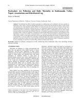
metropolitan areas in the USA for the 7-year period 1987±1994 (Fig. 1 and Table 1). In several
locations, we had a high percentage of days with missing values for PM
10
because it is generally
measured every 6 days. The cause-speci®c mortality data, aggregated at the level of counties,
were obtained from the National Center for Health Statistics. We focused on daily death counts
Air Pollution and Mortality 265
for each site, excluding non-residents who died in the study site and accidental deaths. Because
mortality information was available for counties but not for smaller geographic units to protect
con®dentiality, all predictor variables were aggregated to the county level.
Hourly temperature and dewpoint data for each site were obtained from the EarthInfo
compact disc database. After extensive preliminary analyses that considered various daily
summaries of temperature and dewpoint as predictors, such as the daily average, maximum
and 8-h maximum, we used the 24-h mean for each day. If a city has more than one weather-
station, we took the average of the measurements from all available stations. The PM
10
and
ozone O
3
 data were also averaged over all monitors in a county. To protect against outliers,
a 10% trimmed mean was used to average across monitors, after correction for yearly
averages for each monitor. This yearly correction is appropriate since long-term trends in
mortality are also adjusted in the log-linear regressions. See Kelsall et al. (1997) for further
details. Aggregation strategies based on Bayesian and classical geostatistical models as
suggested by Handcock and Stein (1993), Cressie (1994), Kaiser and Cressie (1993) and
Cressie et al. (1999) and Bayesian models for spatial interpolation (Le et al., 1997; Gaudard
et al., 1999) are desirable in many contexts because they provide estimates of the error
associated with exposure at any measured or unmeasured locations. However, they were not

applicable to our data sets because of the limited number of monitoring stations that are
available in the 20 counties.
3. City-speci®c analyses
In this section, we summarize the model used to estimate the air pollution±mortality relative
rate separately for each location, accounting for age-speci®c longer-term trends, weather and
266 F. Dominici, J. M. Samet and S. L. Zeger
Fig. 1. Map of the 20 cities with largest populations including the surrounding country: the cities are numbered
from 1 to 20 following the order in Table 1
day of the week. The core analysis for each city is a log-linear generalized additive model that
accounts for smooth ¯uctuations in mortality that potentially confound estimates of the
pollution eect and/or introduce autocorrelation in mortality series.
This is a study of the acute health eects of air pollution on mortality. Hence, we modelled
daily expected deaths as a function of the pollution levels on the same or immediately
preceding days, not of the average exposure for the preceding month, season or year as might
be done in a study of chronic eects. We built models which include smooth functions of time
as predictors as well as the pollution measures to avoid confounding by in¯uenza epidemics
which are seasonal and by other longer-term factors.
To specify our approach more completely, let y
c
at
be the observed mortality for each age
group a 465, 65±75, 5 75 years) on day t at location c, and let x
c
at
be a p Â1 vector of air
pollution variables. Let 
c
at
 E y
c

at
 be the expected number of deaths and v
c
at
 vary
c
at
.We
used a log-linear model log
c
at
x
c
H
at

c
for each city c, allowing the mortality counts to have
variances v
c
at
that may exceed their means (i.e. be overdispersed) with the overdispersion
parameter 
c
also varying by location so that v
c
at
 
c


c
at
.
To protect the pollution relative rates 
c
from confounding by longer-term trends due, for
example, to changes in health status, changes in the sizes and characteristics of populations,
seasonality and in¯uenza epidemics, and to account for any additional temporal correlation in
the count time series, we estimated the pollution eect using only shorter-term variations in
mortality and air pollution. To do so, we partial out the smooth ¯uctuations in the mortality
over time by including arbitrary smooth functions of calendar time S
c
(time,  for each city.
Here,  is a smoothness parameter which we prespeci®ed, on the basis of prior epidemiological
knowledge of the timescale of the major possible counfounders, to have 7 degrees of freedom per
year of data so that little information from timescales longer than approximately 2 months is
included when estimating 
c
. This choice largely eliminates expected confounding from seasonal
Air Pollution and Mortality 267
Table 1. Summary by location of the county population Pop, percentage of days with missing values P
missO
3
and P
missPM
10
, percentage of people in poverty P
poverty
, percentage of people older than 65 years P
>65

, average
of pollutant levels for O
3
and PM
10
,
"
X
O
3
and
"
X
PM
10
, and average daily deaths
"
Y
Location (state) Label Pop P
missO
3
P
missPM
10
P
poverty
(%)
P
>65
(%)

"
X
O
3
(parts
per billion)
"
X
PM
(gm
À3
)
"
Y
Los Angeles la 8863164 0 80.2 14.8 9.7 22.84 45.98 148
New York ny 7510646 0 83.3 17.6 13.2 19.64 28.84 191
Chicago chic 5105067 0 8.2 14.0 12.5 18.61 35.55 114
Dallas±Fortworth dlft 3312553 0 78.6 11.7 8.0 25.25 23.84 49
Houston hous 2818199 0 72.9 15.5 7.0 20.47 29.96 40
San Diego sand 2498016 0 82.2 10.9 10.9 31.64 33.63 42
Santa Ana±Anaheim staa 2410556 0 83.6 8.3 9.1 22.97 37.37 32
Phoenix phoe 2122101 0.1 85.1 12.1 12.5 22.86 39.75 38
Detroit det 2111687 36.3 53.9 19.8 12.5 22.62 40.90 47
Miami miam 1937094 1.4 83.4 17.6 14.0 25.93 25.65 44
Philadelphia phil 1585577 0.7 83.1 19.8 15.2 20.49 35.41 42
Minneapolis minn 1518196 100 5.4 9.7 11.6 Ð 26.86 26
Seattle seat 1507319 37.3 24.5 7.8 11.1 19.37 25.25 26
San Jose sanj 1497577 0 67.7 7.3 8.6 17.87 30.35 20
Cleveland clev 1412141 41.4 55.6 13.5 15.6 27.45 45.15 36
San Bernardino sanb 1412140 0 81.6 12.3 8.7 35.88 36.96 20

Pittsburg pitt 1336449 1.3 0.8 11.3 17.4 20.73 31.61 38
Oakland oakl 1279182 0 82.6 10.3 10.6 17.24 26.31 22
San Antonio sana 1185394 0.1 77.1 19.4 9.8 22.16 23.83 20
Riverside river 1170413 0 81.3 14.8 11.3 33.41 51.99 20
in¯uenza epidemics and from longer-term trends due to changing medical practice and health
behaviours, while retaining as much unconfounded information as possible. We also controlled
for age-speci®c longer-term and seasonal variations in mortality, adding a separate smooth
function of time with 8 degrees of freedom for each age group.
To control for weather, we also ®tted smooth functions of the same day temperature
(temp
0
), the average temperature for the three previous days (temp
1 3
, each with 6 degrees of
freedom, and the analogous functions for dewpoint (dew
0
and dew
1 3
, each with 3 degrees of
freedom. In the US cities, mortality decreases smoothly with increases in temperature until
reaching a relative minimum and then increases quite sharply at higher temperature. 6 degrees
of freedom were chosen to capture the highly non-linear bend near the relative minimum as
well as possible. Since there are missing values of some predictor variables on some days, we
restricted analyses to days with no missing values across the full set of predictors.
In summary, we ®tted the following log-linear generalized additive model (Hastie and
Tibshirani, 1990) to obtain the estimated pollution log-relative-rate


c
and the sample co-

variance matrix V
c
at each location:
log
c
at
x
c
H
at

c
 
c
DOW S
c
1
time, 7=yearS
c
2
temp
0
,6S
c
3
temp
1 3
,6
 S
c

4
dew
0
,3S
c
5
dew
1 3
,3intercept for age group a
 separate smooth functions of time 8 degrees of freedom for age group a, 1
where DOW are indicator variables for the day of the week. Samet et al. (1995, 1997) and Kelsall
et al. (1997) give additional details about choices of functions used to control for longer-term
trends and weather. Alternative modelling approaches that consider dierent lag structures of
the pollutants and of the meteorological variables have been proposed (Davis et al., 1996;
Smith et al., 1997, 1998). More general approaches that consider non-linear modelling of the
pollutant variables have been discussed by Smith et al. (1997) and by Daniels et al. (2000).
Because the functions S
c
x,  are smoothing splines with ®xed , the semiparametric
model described above has a ®nite dimensional representation. Hence, the analytical
challenge was to make inferences about the joint distribution of the 
c
s in the presence of
®nite dimensional nuisance parameters, which we shall refer to as 
c
.
We separately estimated three semiparametric regressions for each pollutant with the con-
current day (lag 0), prior day (lag 1) and 2 days prior (lag 2) pollution predicting mortality.
The estimates of the coecients and their 95% con®dence intervals for PM
10

alone and for
PM
10
adjusted by O
3
level are shown in Figs 2 and 3. Cities are presented in decreasing order
by the size of their populations. The pictures show substantial between-location variability
in the estimated relative rates, suggesting that combining evidence across cities would be a
natural approach to explore possible sources of heterogeneity, and to obtain an overall
summary of the degree of association between pollution and mortality. To add ¯exibility in
modelling the lagged relationship of air pollution with mortality, we could have used
distributed lag models instead of treating the lags separately. Although desirable, this is not
easily implemented because many cities have PM
10
data available only every sixth day.
To test whether the log-linear generalized additive model (1) has taken appropriate account
of the time dependence of the outcome, we calculate, for each city, the autocorrelation
function of the standardized residuals. Fig. 4 displays the 20 autocorrelation functions; they
are centred near zero, ranging between À0:05 and 0.05, con®rming that the ®ltering has
removed the serial dependence.
We also examined the sensitivity of the pollution relative rates to the degrees of freedom
used in the smooth functions of time, weather and seasonality by halving and doubling each
268 F. Dominici, J. M. Samet and S. L. Zeger
of them. The relative rates changed very little as these parameters are varied over this fourfold
range (the data are not shown).
4. Pooling results across cities
In this section, we present hierarchical regression models designed to pool the city-speci®c
pollution relative rates across cities to obtain summary values for the 20 largest US cities.
Hierarchical regression models provide a ¯exible approach to the analysis of multilevel data.
In this context, the hierarchical approach provides a uni®ed framework for making estimates

of the city-speci®c pollution eects, the overall pollution eect and of the within- and between-
cities variation of the city-speci®c pollution eects.
The results of several applied analyses using hierarchical models have been published.
Examples include models for the analysis of longitudinal data (Gilks et al., 1993), spatial data
Air Pollution and Mortality 269
Fig. 2. Results of regression models for the 20 cities by selected lag (


c
and 95% con®dence intervals of


c
 1000 for PM
10
; cities are presented in decreasing order by population living within their county limits; the
vertical scale can be interpreted as the percentage increase in mortality per 10 gm
À3
increase in PM
10
): the
results are reported (a) using the concurrent day (lag 0) pollution values to predict mortality, (b) using the previous
day's (lag 1) pollution levels and (c) using pollution levels from 2 days before (lag 2)
(Breslow and Clayton, 1993) and health care utilization data (Normand et al., 1997). Other
modelling strategies for combining information in a Bayesian perspective are provided by Du
Mouchel (1990), Skene and Wake®eld (1990), Smith et al. (1995) and Silliman (1997).
Recently, spatiotemporal statistical models with applications to environmental epidemiology
have been proposed by Wikle et al. (1997) and Wake®eld and Morris (1998).
In Section 4.1 we present an overview of our modelling strategy. In Sections 4.2 and 4.3, we
consider two hierarchical regression models with and without modelling of the possible

spatial autocorrelation among the 
c
s which we refer to as the base-line and spatial models
respectively.
4.1. Modelling approach
The modelling approach comprises two stages. At the ®rst stage, we used the log-linear
generalized additive model (1) described in Section 3:
270 F. Dominici, J. M. Samet and S. L. Zeger
Fig. 3. Results of regression models for the 20 cities by selected lag (


c
and 95% con®dence intervals of


c
 1000 for PM
10
adjusted by O
3
level; cities are presented in decreasing order by population living within their
county limits; the empty symbol at Minneapolis represents the missingness of the ozone data in this city; the
vertical scale can be interpreted as the percentage increase in mortality per 10 gm
À3
increase in PM
10
): the
results are reported (a) using the concurrent day (lag 0) pollution values to predict mortality, (b) using the previous
day's (lag 1) pollution levels and (c) using pollution levels from 2 days before (lag 2)
y

c
t
j
c
, 
c
$ Poisson f
t

c
, 
c
g
where y
c
t
y
c
465t
, y
c
65 75t
, y
c
575t
. The parameters of scienti®c interest are the mortality relative
rates 
c
, which for the moment are assumed not to vary across the three age groups within a
city. The vector 

c
of the coecients for all the adjustment variables, including the splines in
the semiparametric log-linear model, is a ®nite dimensional nuisance parameter.
The second stage of the model describes variation among the 
c
s across cities. We regressed
the true relative rates on city-speci®c covariates z
c
to obtain an overall estimate, and to
explore the extent to which the site-speci®c explanatory variables explain geographic vari-
ation in the relative risks. In epidemiological terms, the covariates in the second stage are
possible eect modi®ers. More speci®cally, we assumed

c
j, Æ $ N
p
z
c
, Æ
where p is the number of pollutant variables that enter simultaneously in model (1). Here the
parameters of scienti®c interest are the vector of the regression coecients, , and the overall
covariance matrix Æ. Unlike the overall air pollution eect , we are not interested in
estimating overall non-linear adjustments for trend and weather; therefore we assume that
the nuisance parameters 
c
are independent across cities. Our goal is to make inferences
about the parameters of interest Ð the 
c
s,  and Æ Ð in the presence of nuisance parameters


c
. To estimate an exact Bayesian solution to this pooling problem, we could analyse the joint
Air Pollution and Mortality 271
Fig. 4. Plots of city-speci®c autocorrelation functions of standardized residuals r
t
, where r
t
 (Y
t
À

Y
t
)=
p

Y
t
and

Y
t
are the ®tted values from log-linear generalized additive model (1)
posterior distributions of the parameters of interest, as well as of the nuisance parameters,
and then integrate over the 
c
-dimension to obtain the marginal posterior distributions of the

c
s. Although possible, the computations become extremely laborious and are not practical

for either this analysis or a planned model with 90 or more cities.
Given the large sample size at each city (T ranges from 550 to 2550 days), accurate approx-
imations to the posterior distribution can be obtained by using the normal approximation of
the likelihood (Le Cam and Yang, 1990). If the likelihood function of 
c
and 
c
is approx-
imated by a multivariate normal distribution with mean equal to the maximum likelihood
estimates


c
and 
c
and covariance matrices V

and V

, then by de®nition the marginal
likelihood of 
c
has a multivariate normal distribution with mean


c
and covariance matrix
V

. We then replaced the ®rst stage of the model with a normal distribution with mean and

variance equal to the maximum likelihood estimates of the parameter. Recently it has been
shown that the strategy based on the normal approximation of the likelihood gives an
alternative two-stage model that well approximates the original model and leads to more
ecient simulation from the posterior (Daniels and Kass, 1998).
To check whether inferences based on the normal approximation of the likelihood are
proper, we compared our approach with the implementation of the full Markov chain Monte
Carlo approach for a few cities with sample sizes ranging from 2000 in Pittsburgh to 545 in
Riverside. Fig. 5 shows the histogram of samples for Riverside from p 
c
jdataÐ obtained
by implementing a Gibbs sampler that simulates from p
c
j
c
, data) and p
c
j
c
, data) and
approximate
p
c
jdata

p
c
, 
c
jdatad
c

Ð with samples from N 


c
, V
c
 (full curve). The two distributions are very similar.
4.2. Base-line model
Let 
c

c
PM
10
, 
c
O
3

H
be the log-relative-rate associated with PM
10
and O
3
level at city c.We
considered the hierarchical model


c
j

c
$ N
2

c
, V
c
,

c
PM
10
 z
c
H
PM
10

PM
10
 
c
PM
10
,

c
O
3
 z

c
H
O
3

O
3
 
c
O
3
,

c
jÆ $ N
2
0, Æ
9
>
>
>
>
>
=
>
>
>
>
>
;

2
where z
c
PM
10
1, P
c
poverty
, P
c
>65
,
"
X
c
PM
10

H
, z
c
O
3
1, P
c
poverty
, P
c
>65
,

"
X
c
O
3

H
, 
PM
10
and 
O
3
are 4 Â1
vectors and ®nally 
c

c
PM
10
, 
c
O
3

H
, c  1, . . ., 20. This model speci®cation allowed a
dependence between the relative rates associated with PM
10
and O

3
level, but implied inde-
pendence between the relative rates of cities c and c
H
.
Under this model, the true PM
10
and O
3
log-relative-rates in city c were regressed on
predictor variables including the percentage of people in poverty P
c
poverty
 and the percentage
of people older than 65 years (P
c
>65
), and on the average of the daily values of PM
10
and O
3
level over the period 1987±1994 in location c (
"
X
c
PM
10
and
"
X

c
O
3
. If we centred the predictors
about their means, the intercepts 
0,PM
10
and 
0,O
3
can be interpreted as overall eects for a
city with mean predictors. A simple pooled estimate of the pollution eect is obtained by
setting all covariates to 0. To compare the consequences of considering two pollutants
272 F. Dominici, J. M. Samet and S. L. Zeger
independently and jointly in the model, we ®t a base-line±univariate model Ð i.e. Æ assumed
diagonal Ð and a base-line±bivariate model Ð i.e. Æ assumed to have non-zero o-diagonal
elements.
Inference on the parameters  
PM
10
, 
O
3

H
and Æ represents a synthesis of the informa-
tion from the 20 cities; for example the parameters 
0j
, Æ 
jj

, j  PM
10
,O
3
, determine the
overall level and the variability of the relative change in the rate of mortality associated with
changes in the jth pollutant level on average over all the cities.
The Bayesian formulation was completed by specifying dispersed but proper base-line
prior distributions and then supplementing the base-line analysis with additional sensitivity
analysis. A priori, we assumed that the joint prior is the product of the marginals for  and Æ.
The following base-line prior speci®cations for the marginals are used:
overall log-relative-rates  $ N
pk1
m, V

,
overall covariance matrix Æ $ IW
p
df, D
where IW
p
df, D denotes the inverse Wishart distribution with df degrees of freedom and
scale matrix D,ap Âp positive de®nite matrix, whose density is proportional to
Air Pollution and Mortality 273
Fig. 5. Comparison between the normal approximation of the likelihood of 
c
and the marginal posterior
distribution of 
c
:

Ð
, normal density N(


c
, V
c
) where


c
and V
c
are the maximum likelihood estimates
of a semiparametric Poisson regression model; histogram, marginal posterior distribution of 
c
obtained by
implementing a full Gibbs sampler for the parameter of interest 
c
and for the coef®cients of the natural cubic
splines 
c
D
dfpÀ1=2
jÆj
df2p=2
exp

À
1

2
trDÆ
À1


:
Here p denotes the number of pollutant variables entering the model simultaneously and k
the number of city-speci®c covariates. We select m equal to a vector of 0s, V

equal to a
diagonal matrix, with diagonal elements equal to 100, df  3 and D a diagonal matrix with
diagonal elements equal to 3. In the univariate case we denote Æ by 
2
. These prior hyper-
parameters lend prior 95% support to the overall eect, the city-speci®c eects and the
correlation between the PM
10
and the O
3
log-relative-rates equal to À15, 15), À4, 4) and
À0:85, 0.85) respectively. This prior speci®cation was selected because it did not impose too
much shrinkage of the study-speci®c parameters towards their overall means, while specifying
a reasonable range for the unknown parameters a priori. A sensitivity analysis is presented in
Table 4 in Section 5.
Given these prior assumptions, we can draw inferences on the unknown parameters by
using the posterior distribution
p
1
, ,
20

, , Æj


1
, ,


20
, V
1
, ,V
20
: 3
To do this, we implemented a Markov chain Monte Carlo algorithm with a block Gibbs
sampler (Gelfand and Smith, 1990) in which the unknowns are partitioned into the groups

c
,  and Æ. Each group is sampled in turn, given all others. The full conditional distri-
butions were available in closed form. Their derivation was routine (Bernardo and Smith,
1994) and is not detailed here. Because of the normality assumptions at the ®rst and second
stage of the hierarchical model, computations of the posterior distributions of all the
unknowns under a univariate model can be performed via direct simulation following the
factorization above:
p 
1
, ,
20
, , 
2
jdatap

2
jdata pj
2
, data
Q
c
p 
c
j, 
2
, data.
The ®rst step, simulating 
2
, can be performed numerically (using the inverse cumulative
density function method, for example). The second and third steps can be done easily by
sampling from normal distributions. This strategy can be conveniently implemented only for
the univariate base-line model.
4.3. Spatial model
The assumption of independence of the city-speci®c coecients that is made in the base-line
model can be relaxed to a more general model in which the correlation between 
c
and 
c
H
decays as either a smooth or step function to 0 as the distance between the two cities, c and c
H
,
increases. In this section, we consider a hierarchical model in which the inferences allow for
the possible spatial correlation among the 
c

s. We only considered univariate models given
the small number of cities; an extension to multivariate models is straightforward but requires
a larger data set.
At the second stage of the spatial model, we assumed that there is a systematic variation in
the air pollution±mortality relationship from pollutant to pollutant as speci®ed in the base-
line model (2). We expressed the degree of similarity of the relative rates in locations c and c
H
as a function of an (arbitrary) distance between c and c
H
, by assuming c, c
H
corr
c
, 
c
H

 expfÀ dc, c
H
g. We considered two distance measures, the Euclidean distance between
the cities c and c
H
in the longitude and latitude co-ordinates and a step function such
274 F. Dominici, J. M. Samet and S. L. Zeger
that dc, c
H
1 if locations c and c
H
are within a common `region' and dc, c
H

Iif not. To
make the results of these two models comparable we rescaled the Euclidean distance such that
it ranges between 0 and 4 with median equal to 0.64. The spatial model with (1, I distance
can also be speci®ed as a three-stage hierarchical model where the ®rst stage is as the base-line
model (2), the second stage describes the heterogeneity of the estimates across cities within
regions and the third stage describes the heterogeneity of the estimates across regions. For this
regional model, we have clustered the 20 cities in the following three regions: north-east,
south-east and west coast. Thus, if we indicate by 
2
the variability of the estimates across
regions and by 
2
the variability of the estimates within regions, then the correlation of the
log-relative-rates for locations c and c
H
within a common region is 
2
=
2
 
2
. Alternative
de®nitions of distance can be incorporated easily into the model as appropriate.
The spatial model speci®cation is completed with the elicitation of the prior distribution.
For  and 
2
we choose the same prior speci®ed in Section 4.2. For the parameter  under
the spatial model with Euclidean distance, we choose a log-normal prior with mean 0.2 and
standard deviation 0.5. Let
~

d be the median of the distribution of all distances; this speci-
®cation leads to a prior distribution of the correlation expÀ
~
d  having mean 0.45 (95%
interval: 0.11, 0.74). For the parameter 
2
under the spatial model with step distance, we chose
an inverse gamma prior IGA, B with parameters A  5andB  8:5. This speci®cation leads
to a prior distribution for  having mean 1.35 (95% prior interval: 0.9, 2.2) and a prior
distribution for the correlation 
2
=
2
 
2
 having mean 0.45 (95% prior interval: 0.13, 0.77).
In the spatial model, the full conditionals for 
c
,  and 
2
are all available in closed form.
In contrast, to sample from the full conditional distribution of , we used a Metropolis±
Hastings algorithm with a gamma proposal distribution having mean equal to the current
value of  and ®xed variance. The spatial model with a step distance can be more eciently
sampled with a block Gibbs sampler because the full conditional distributions of all the
unknown parameters are available in closed form.
5. Results
We ran the Gibbs sampler for 3000 iterations for both the base-line and the spatial models,
ignoring the ®rst 100. The autocorrelation, computed from a random sample of the 
0,PM

10
,is
negligible at lag 5 so we sampled every ®fth observations for posterior estimation. The accep-
tance probabilities for the Metropolis algorithm averaged between 0.3 and 0.5. Convergence
diagnosis was performed by implementing Raftery and Lewis's (1992) methods in CODA (Best
et al., 1995) which reported the minimum number of iterations N
min
needed to estimate the
variable of interest with an accuracy of Æ0:005 and with probability of attaining this degree of
accuracy equal to 0.95. N
min
9 2000 are proposed.
Fig. 6 summarizes results of the pooled analyses under the univariate±base-line model. It
displays the posterior distributions of city-speci®c regression coecients 
c
associated with
changes in PM
10
-measurements for the 20 cities at the current day, 1-day lag and 2-day lag.
The marginal posterior distribution of the overall eect 
0,PM
10
 is displayed at the far right-
hand side. Cities are ordered by the decreasing size of their populations. At the current day,
the highest relative rate for the PM
10
-variable occurs in New York with a 1.05% increase
in mortality (95% interval: 0.5, 1.6) per 10 gm
À3
increase in PM

10
. Overall, we found that a
10 gm
À3
increase in PM
10
is associated with an estimated 0.48% increase in mortality (95%
interval: 0.05, 0.92).
Fig. 7 summarizes the results of the pooled analyses under the bivariate±base-line model.
When PM
10
and O
3
level are combined in the same model, we estimated that 10-unit
Air Pollution and Mortality 275
increments in PM
10
adjusted by O
3
are associated with mortality increases of 0.52% (95%
interval: 0.16, 0.85).
The marginal posterior distribution of the overall regression eect combined and synthesized
the information from the 20 locations. Fig. 8 shows the marginal posterior distributions of
the overall pollution relative rates at the current day, 1-day and 2-day lags obtained from the
base-line±univariate, base-line±bivariate and spatial models. At the top right-hand side are
summarized the posterior probabilities that the overall eects are larger than 0 for each lag
speci®cation. In the univariate and bivariate analyses, we found signi®cant eects of PM
10
.
Results of the adjusted analyses under the univariate±base-line model are shown in Table

2. Here we summarize the posterior means and the 95% posterior support intervals for the
276 F. Dominici, J. M. Samet and S. L. Zeger
Fig. 6. Results of pooled analyses under the univariate±base-line model (PM
10
entered independently in the
model) (box plots of samples from the posterior distributions of city-speci®c regression coef®cients 
c
associated
with changes in PM
10
-measurements; for comparison, samples from the marginal posterior distribution of the
corresponding overall effects are displayed at the far right-hand side; the vertical scale can be interpreted as the
percentage increase in mortality per 10 gm
À3
increase in PM
10
): the results are reported (a) using the concurrent
day (lag 0) pollution values to predict mortality, (b) using the previous day's (lag 1) pollution levels and (c) using
pollution levels from 2 days before (lag 2)
relationship between the mean of the city-speci®c coecients and the percentage in poverty,
the percentage of people older than 65 years and the mean level of the pollutant. Here the
intercept 
0
denotes the overall eect of PM
10
with mean predictors. None of these variables
are found to predict the PM
10
relative rate.
An interaction of the pollution eects and age could be detected by the coecient of the

variable P
>65
in the second-stage regression model. A more direct approach was to estimate a
separate pollution relative rate for each age stratum in the ®rst-stage log-linear models and
then to pool the trivariate vector 


<65
,


65 75
,


>75
 across cities. When we did so, the estimates
of the overall eect of PM
10
for the three age groups have posterior means 0.63 (95%
interval: 0.24, 1.05), 0.26 (95% interval: À0:14, 0.67) and 0.46 (95% interval: 0.04, 0.83).
Air Pollution and Mortality 277
Fig. 7. Results of pooled analyses under the bivariate±base-line model (PM
10
and O
3
level entered
simultaneously in the model) (box plots of samples from the posterior distributions of city-speci®c regression
coef®cients 
c

associated with changes in PM
10
adjusted by O
3
measurements; for comparison, samples from the
marginal posterior distribution of the corresponding overall effects are displayed at the far right-hand side; the
vertical scale can be interpreted as the percentage increase in mortality per 10 gm
À3
increase in PM
10
respectively): the results are reported (a) using the concurrent day (lag 0) pollution values to predict mortality, (b)
using the previous day's (lag 1) pollution levels and (c) using pollution levels from 2 days before (lag 2)
278 F. Dominici, J. M. Samet and S. L. Zeger
Fig. 8. Results of pooled analyses under (a) the univariate±base-line, (b) bivariate±base-line and (c) spatial
models (marginal posterior distributions of the overall effects, 
0,PM
10
, for various lags; at the top right-hand side
are speci®ed the posterior probabilities that the overall effects are larger than 0)
These results suggest that there is no trend in the pollution relative rates with age as is
suggested by the second-stage regression results in Table 2.
The variability of the regression coecients, on average, over all the locations was
captured by the matrix Æ. Marginal posterior means and 95% posterior support intervals are
summarized in Table 3. A large diagonal element signi®ed large variability over cities in the
corresponding coecient, whereas a large o-diagonal element signi®es strong correla-
tion between the PM
10
- and O
3
coecients. Table 3 shows the results. Under the base-line±

univariate model, the standard deviation of the true coecients across cities was estimated to
be 0.76 (95% interval: 0.41, 1.37) which is about twice as large as the overall estimate of the
pollution eect. Hence, in univariate analyses, the variability in the PM
10
-coecient is non-
negligible. The posterior distribution of the o-diagonal elements of Æ indicates a negative
mean correlation between the eects of the two pollutants, but with a large standard deviation.
From the posterior samples of  in the spatial model, we could easily calculate the marginal
posterior distributions of the correlation coecient c, c
H
expfÀ d c, c
H
gfor each distance
dc, c
H
. For the cities having median distance, the posterior mean correlation between 
c
and

c
H
was 0.61 (95% interval: 0.3, 0.8). Consider the 25% and 75% quantiles of the distribution
of all distances. Each of these quantiles has an associated correlation coecient. The
posterior means of these two correlation coecients were 0.86 (95% interval: 0.68, 0.93) and
0.3 (95% interval: 0.05, 0.58), both larger than the corresponding prior means.
Under the regional model, with distance equal to a step function, the posterior mean of
the within-region correlation of the city-speci®c relative rates 
2
=
2

 
2
 was 0.68 (95%
interval: 0.42, 0.86). Results for the PM
10
eects under the two spatial models were similar
Air Pollution and Mortality 279
Table 2. Results of the second-stage analyses under the base-line±univariate model (PM
10
entered independently in the model){
City-specific
covariate
Posterior means and support intervals for the following lags:
Lag 0 Lag 1 Lag 2
Overall PM
10
0.40 (70.06, 0.85) 0.52 (0.06, 0.98) 0.43 (70.03, 0.87)
P
poverty
(%) 70.08 (70.21, 0.04) 70.01 (70.14, 0.11) 70.01 (70.11, 0.12)
P
>65
(%) 70.01 (70.19, 0.17) 0.03 (70.15, 0.20) 0.00 (70.16, 0.17)
"
X
c
PM
10
(gm
À3

) 0.02 (70.05, 0.08) 70.01 (70.07, 0.06) 0.01 (70.05, 0.07)
{Posterior means and 95% posterior support intervals of the coecients for the relationship
between the true relative rate 
c
, the percentage in poverty P
poverty
, the percentage of people older
than 65 years P
>65
and the mean level of the pollutant
"
X
PM
10
. The results are reported using the
concurrent day (lag 0) pollution values to predict mortality, using the previous day's (lag 1)
pollution levels and using pollution levels from 2 days before (lag 2).
Table 3. Posterior means and 95% support intervals of the elements of Æ under the three
models (univariate, bivariate and spatial)
Model Posterior means and support intervals for the following effects{:
std of PM
10
effects std of O
3
effects corr of PM
10
and O
3
effects
Base-line±bivariate 0.36 (0.17, 0.75) 0.91 (0.33, 2.01) 70.09 (70.5, 0.22)

Base-line±univariate 0.76 (0.41, 1.37) 1.28 (0.69, 2.28)
Spatial 0.71 (0.38, 1.27) 1.21 (0.61, 2.32)
{std of PM
10
eects, standard deviation across locations of the 
c
PM
10
; std of O
3
eects, standard
deviation across locations of the 
c
O
3
; corr of PM
10
and O
3
eects, correlation between the 
c
PM
10
and 
c
O
3
.
qualitatively. The posterior means and interquartile range for the regional eects 
east

, 
south
and

west
are 0.40 (À0:22, 1.03), À0:06 (À0:96, 0.93) and 0.69 (0.07, 1.35), revealing that the adverse
health eects of PM
10
on mortality in the west of the USA is larger than in the east and south.
We have assessed the robustness of the results with respect to choices of the model (uni-
variate, bivariate and spatial), of the lag structure (lag 0, lag 1 and lag 2) and of the prior
distributions. Our sensitivity analysis compared 27 alternative scenarios (three for model
choice, three for lag structures and three for prior distributions). For these scenarios we
compare the posterior probability that the overall eect of PM
10
is larger than 0. The con-
sequences of these choices are shown in Table 4. Signi®cant eects of PM
10
on total daily
mortality are observed in all three models (but weaker under a spatial model with current day
pollution predicting mortality). When both pollutants are included in the model, adverse
eects of PM
10
became stronger. Spatial analyses attenuate the eects.
6. Discussion
We have developed a statistical model for obtaining a national estimate of the eect of urban
air pollution on daily mortality using data for the 20 largest US cities. The raw data com-
prised publicly available listings of individual deaths by day and location, and hourly
measurements of pollutants and weather variables. Substantial preprocessing of the nearly
1 Gbyte of information is necessary to create daily time series of mortality, pollutants and

weather for each of the 20 cities.
Because the estimation of a national pollution relative rate is the primary objective of this
study, a two-stage approach was developed that allowed the modelling eort to focus on
combining information across cities. In the ®rst stage, a log-linear regression is used to
estimate a pollution relative rate for each city while controlling for the city-speci®c longer-
term time trends and weather eects. Because we had no speci®c scienti®c interest in the time
or weather eects, no eort is made to impose modelling assumptions to enable borrowing
strength across cities when estimating the eects on mortality of these variables.
In the second stage, we regressed the true relative rates on city-speci®c covariates to obtain
an overall estimate, and to estimate the variation among the coecients across cities. We then
generated posterior estimates of the overall pollution eect and of the city-speci®c eects by
using Markov chain Monte Carlo methods. Four models for combining relative rates of
mortality for PM
10
across cities were used. In the ®rst, relative rates from dierent cities are
treated as independent of one another. In the second, relative rates from dierent cities are
treated as independent of one another, but are adjusted by O
3
level. In the third and fourth
280 F. Dominici, J. M. Samet and S. L. Zeger
Table 4. Posterior probabilities that the overall effects of PM
10
are larger than 0 by lag and by three
prior distributions under the three models (univariate, bivariate and spatial)
Model Posterior probabilities for the following priors and lags{:
Prior 1 Prior 2 Prior 3
Lag 0 Lag 1 Lag 2 Lag 0 Lag 1 Lag 2 Lag 0 Lag 1 Lag 2
Base-line±univariate 0.98 0.98 0.99 0.98 0.96 0.98 0.95 0.96 0.93
Base-line±bivariate 1 1 0.97 1 0.99 0.99 0.98 1 0.93
Spatial 0.83 0.95 0.92 0.83 0.93 0.91 0.78 0.89 0.85

{The three prior speci®cations have the following 95% support intervals of the overall eects, the city-speci®c
eects and of the spatial correlation for the relative rates of the two closest cities with median distance: prior 1,
(À15, 15), (À4, 4), (0.11, 0.74); prior 2, (À4, 4), (À4, 4), (0.11, 0.74); prior 3, À4, 4), (À7, 7), (0, 0.9).
models the possibility of geographic correlation between the true coecients is allowed.
Results under the four models are similar: bivariate analyses give slightly higher eects and
spatial analyses slightly attenuate the eects. Results under dierent models, lag speci®ca-
tions and priors are summarized in Fig. 8 and Table 4. Note that the variance of the posterior
distribution of the overall relative rate in the spatial models is somewhat sensitive to the prior
speci®cation for the between-region variance or equivalently within-region correlation since,
with our 20 cities, we have only three regions and hence limited information. A similar
analysis of the 90 largest cities will provide more precise information about variation across
regions.
These analyses demonstrated that there was a consistent association of particulate air
pollution PM
10
with daily mortality across the 20 largest US cities leading to an overall eect,
which was positive with high probability. Our overall estimate was that an increase of 10 gm
À3
in particulate level is associated with a roughly 0.48% increase in daily mortality on that day
or the next day.
Another multicity study of air pollution and mortality is the multicentre European study,
`Air pollution and health: a European approach' (Katsoyanni et al., 1997; Toulomi et al.,
1997). The cities were selected from across Europe, although not systematically. Data on
particulate air pollution and daily mortality are analysed from 12 cities from western and
central Europe according to a standardized protocol. Model estimates from the individual
cities are pooled as the weighted means of the regression coecients and heterogeneity
among cities is explored using a random-eects model. For particulate matter, the ®ndings
diered between the western and central Europe cities, with a ®vefold greater eect in the
western cities (Katsoyanni et al., 1997). A similar approach is applied to the six selected cities
with data available on O

3
. A signi®cant eect of O
3
is found, after controlling for levels of
black smoke and an index of particulate matter (Toulomi et al., 1997).
Although it is only a ®rst step, the modelling described here establishes a basis for carry-
ing out national surveillance for eects of air pollution and weather on public health. The
analyses could be easily extended to studies of cause-speci®c mortality and other pollutants.
Monitoring eorts using models like that described here would be appropriate given the
important public health questions that they can address and the considerable expense to
government agencies for collecting the information that forms the basis for this work.
An alternative modelling strategy would have been to use one large Markov chain Monte
Carlo method to estimate simultaneously the parameters in the log-linear models within each
city, the overall estimate of the pollutant and all the nuisance parameters, borrowing strength
across cities to obtain more precise estimates of the nuisance functions for each city. This type
of approach would be necessary if there were limited information about the nuisance param-
eters within each city as, for example, in the Neyman and Scott problem (Neyman and Scott,
1960). As this is not the case in our investigation, we focused the modelling and computing
eort on combining city-speci®c relative rate estimates to obtain a national average relative
rate.
If the likelihood function for the pollution relative rate and the nuisance parameters is well
approximated by a Gaussian distribution, then our approach will give a close approximation
to the posterior distribution from a Markov chain Monte Carlo sample that simulated both
the parameters of interest and the nuisance parameters. We compared the marginal posterior
of the 
c
obtained by using a full Markov chain Monte Carlo procedure with our normal
approximation for a few cities; they are indistinguishable.
The approach of taking a weighted average of the city-speci®c estimates to obtain an
estimate of the overall eect, as for example suggested by DerSimonian and Laird (1986), is a

Air Pollution and Mortality 281
simpli®ed version or approximation to the use of hierarchical models with a Gibbs sampler.
Under the weighted average approach for a random-eect model, the weights of the city-
speci®c estimates are modi®ed to take into account the variability between locations, say 
2
,
and an estimate of this variance is included. Rather than including a single estimate of 
2
, the
Bayesian method permits incorporating the whole posterior distribution of 
2
. In this way, all
the information about the variability between studies is considered. In addition, the Bayesian
method provides estimates of the posterior distribution of the city-speci®c relative rates and
of the national estimate, and it easily lends itself to generating ranking probabilities as, for
example, P(overall log-relative-rate 5 0j data. In addition, the Gibbs sampler is necessary
for approximating the posterior distributions under the spatial model.
These analyses alone cannot establish that increased levels of particulate air pollution as
measured by PM
10
cause an increase in mortality. They do, however, establish that there is a
consistent association between shorter-term variations in PM
10
and shorter-term variations in
mortality, and that this association is very unlikely to be explained by the eects of longer-
term confounders such as a change in medical practice, in¯uenza epidemics or seasonality,
which have been controlled for by using a city-speci®c adjustment for longer-term trends.
Nor can these associations be explained by confounding eects of temperature or dewpoint
temperature, which again have been controlled for by using city-speci®c adjustment methods.
Acknowledgements

The research described in this paper was conducted under contract to the Health Eects
Institute (HEI), an organization jointly funded by the Environmental Protection Agency
(EPA) (grant R824835) and automotive manufacturers. The contents of this paper do not
necessarily re¯ect the views and policies of the HEI; nor do they necessarily re¯ect the views
and policies of the EPA, or motor vehicles or engine manufacturers. The authors are grateful
to Dr Giovanni Parmigiani and Dr Frank Curriero for comments on an earlier draft and to
Ivan Coursac and Jing Xu for development of the database.
References
American Thoracic Society (1996a) Health eects of outdoor air pollution, part 1. Am. J. Resp. Crit. Care Med., 153,
3±50.
Ð
(1996b) Health eects of outdoor air pollution, part 2. Am. J. Resp. Crit. Care Med., 153, 477±498.
Bernardo, J. M. and Smith, A. F. M. (1994) Bayesian Theory. New York: Wiley.
Best, N. G., Cowles, M. K. and Vines, K. (1995) CODA: convergence diagnostics and output analysis software for
Gibbs sampling output, version 0.30. Technical Report. Medical Research Council Biostatistics Unit, Cambridge.
Breslow, N. and Clayton, D. (1993) Approximation inference in generalized linear mixed models. J. Am. Statist. Ass.,
88, 9±25.
Carroll, R. J., Ruppert, D. and Stefanski, L. (1995) Measurement Error in Nonlinear Models. New York: Chapman
and Hall.
Clyde, M. (1998) Bayesian model averaging and model search strategies. In Bayesian Statistics 6 (eds J. M. Bernardo,
J. O. Berger, A. P. Dawid and A. F. M. Smith), pp. 83±102. Oxford: Oxford University Press.
Cressie, N. (1994) Statistics for Spatial Data. New York: Wiley.
Cressie, N., Kaiser, M., Daniels, M., Aldworth, J., Lee, J., Lahiri, S. and Cox, L. (1999) Spatial analysis of
particulate matter in an urban environment. In Proc. GeoEnv 98 (eds J. Gomez-Hernandez, A. Soares and
R. Froidevaux).
Daniels, M., Dominici, F. and Samet, J. (2000) Estimating PM
10
-mortality dose-response curves and threshold levels:
an analysis of daily time-series for the 20 largest US cities. Am. J. Epidem., to be published.
Daniels, M. and Kass, R. (1998) A note on ®rst-stage approximation in two-stage hierarchical models. Sankhya B,

60, 19±30.
Davis, J., Sacks, J., Saltzman, N., Smith, R. and Styer, P. (1996) Airborne particulate matter and daily mortality in
Birmingham, Alabama. Technical Report. National Institute of Statistical Science, Research Triangle Park.
282 F. Dominici, J. M. Samet and S. L. Zeger
DerSimonian, R. and Laird, N. (1986) Meta-analysis in clinical trials. Contr. Clin. Trials, 7, 177±188.
Dockery, D. and Pope, C. (1994) Acute respiratory eects of particulate air pollution. A. Rev. Publ. Hlth, 15, 107±132.
Dominici, F., Zeger, S. and Samet, J. (2000) A measurement error correction model for time-series studies of air
pollution and mortality. Biostatistics, 2, in the press.
DuMouchel, W. H. (1990) Bayesian metaanalysis. In Statistical Methodology in the Pharmaceutical Sciences (ed.
D. A. Berry), pp. 509±529. New York: Dekker.
DuMouchel, W. H. and Harris, J. E. (1983) Bayes methods for combining the results of cancer studies in humans and
other species. J. Am. Statist. Ass., 78, 293±308.
Fung, Y. and Krewski, D. (1999) On measurement error adjustment methods in poisson regression. Environmetrics,
10, 213±224.
Gaudard, M., Karson, M., Linder, E. and Sinha, D. (1999) Bayesian spatial prediction. Environ. Ecol. Statist., 6,
147±171.
Gelfand, A. E. and Smith, A. F. M. (1990) Sampling-based approaches to calculating marginal densities. J. Am.
Statist. Ass., 85, 398±409.
Geman, S. and Geman, D. (1993) Stochastic relaxation, Gibbs distributions and the Bayesian restoration of images.
J. Appl. Statist., 20, 25±62.
Gilks, W. R., Clayton, D. G., Spiegelhalter, D. J., Best, N. G., McNeil, A. J., Sharples, L. D. and Kirby, A. J. (1993)
Modelling complexity: applications of Gibbs sampling in medicine. J. R. Statist. Soc. B, 55, 39±52.
Handcock, M. and Stein, M. (1993) A bayesian analysis of kriging. Technometrics, 35, 403±410.
Hastie, T. J. and Tibshirani, R. J. (1990) Generalized Additive Models. New York: Chapman and Hall.
Hastings, W. K. (1970) Monte Carlo sampling methods using Markov chains and their applications. Biometrika, 57,
97±109.
Janssen, N., Hoek, G., Brunekreef, B., Harssema, H., Mensink, I. and Zuidhof, A. (1998) Personal sampling of
particles in adults: relation among personal, indoor, and outdoor air concentrations. Am. J. Epidem., 147, 537±544.
Janssen, N., Hoek, G., Harssema, H. and Brunekreef, B. (1997) Childhood exposure to PM10: relation between
personal, classroom, and outdoor concentrations. Occup. Environ. Med., 54, 1±7.

Kaiser, M. and Cressie, N. (1993) The construction of multivariate distributions from markov random ®elds. J.
Multiv. Anal., 2, 35±54.
Katsoyanni, K., Toulomi, G., Spix, C., Balducci, F., Medina, S., Rossi, G., Wojtyniak, B., Sunyer, J., Bacharova, L.,
Schouten, J., Ponka, A. and Anderson, H. R. (1997) Short term eects of ambient sulphur dioxide and particulate
matter on mortality in 12 European cities: results from time series data from the APHEA project. Br. Med. J., 314,
1658±1663.
Kelsall, J., Samet, J. and Zeger, S. (1997) Air pollution, and mortality in Philadelphia, 1974±1988. Am. J. Epidem.,
146, 750±762.
Korrick, S., Neas, L., Dockery, D. and Gold, D. (1998) Eects of ozone and other pollutants on the pulmonary
function of adult hikers. Environ. Hlth Perspect., 106, 93±99.
Le, N. D., Sun, W. and Zidek, J. V. (1997) Bayesian multivariate spatial interpolation with data missing by design. J.
R. Statist. Soc. B, 59, 501±510.
Le Cam, L. and Yang, G. L. (1990) Asymptotics in Statistics: Some Basic Concepts. New York: Springer.
Li, Y. and Roth, H. (1995) Daily mortality analysis by using dierent regression models in Philadelphia county,
1973±1990. Inhaln Toxicol., 7, 45±58.
Liang, K Y. and Zeger, S. L. (1986) Longitudinal data analysis using generalized linear models. Biometrika, 73,13±22.
Lindley, D. V. and Smith, A. F. M. (1972) Bayes estimates for the linear model (with discussion). J. R. Statist. Soc. B,
34, 1±41.
Lioy, P., Waldman, J., Buckley, T., Butler, J. and Pietarinen, T. (1990) The personal, indoor, and outdoor
concentrations of PM10 measured in an industrial community during the winter. Atmos. Environ., 24, 57±66.
Lipfert, F. and Wyzga, R. (1993) Air pollution and mortality: issues and uncertainty. J. Air Waste Mangmnt Ass., 45,
949±966.
Mage, T. and Buckley, T. J. (1995) The relationship between personal exposures and ambient concentrations of
particulate matter. In Air and Waste Management 88th A. Meet., Pittsburgh, pp. 1±16.
Morris, C. N. and Normand, S L. (1992) Hierarchical models for combining information and for meta-analysis. In
Bayesian Statistics 4 (eds J. M. Bernardo, J. O. Berger, A. P. Dawid and A. F. M. Smith), pp. 321±344. Oxford:
Oxford University Press.
Neyman, J. and Scott, E. L. (1960) Correction for bias introduced by a transformation of variables. Ann. Math.
Statist., 31, 643±655.
Normand, S., Glickman, M. and Gatsonis, C. (1997) Statistical methods for pro®ling providers of medical care:

issues and applications. J. Am. Statist. Ass., 92, 803±814.
Ozkaynak, H., Xue, J., Spengler, J., Wallace, L., Pellizzari, E. and Jenkins, P. (1996) Personal exposure to airborne
particles and metals: results from the particle team study in Riverside, California. J. Expos. Anal. Environ.
Epidem., 6, 57±78.
Raftery, A. and Lewis, S. (1992) How many iterations in the gibbs sampler? In Bayeisan Statistics 4 (eds J. M.
Bernardo, J. O. Berger, A. P. Dawid and A. F. M. Smith), pp. 763±774. Oxford: Oxford University Press.
Air Pollution and Mortality 283
Samet, J., Zeger, S. and Berhane, K. (1995) The Association of Mortality and Particulate Air Pollution. Cambridge:
Health Eects Institute.
Samet, J., Zeger, S., Kelsall, J., Xu, J. and Kalkstein, L. (1997) Air pollution, weather and mortality in Philadelphia.
In Particulate Air Pollution and Daily Mortality: Analyses of the Eects of Weather and Multiple Air Pollutants, the
Phase IB Report of the Particle Epidemiology Evaluation Project. Cambridge: Health Eects Institute.
Schwartz, J. (1995) Air pollution and daily mortality in Birmingham, Alabama. Am. J. Epidem., 137, 1136±1147.
Silliman, N. (1997) Hierarchical selection models with applications in meta-analysis. J. Am. Statist. Ass., 92, 926±936.
Skene, A. M. and Wake®eld, J. C. (1990) Hierarchical models for multicentre binary response studies. Statist. Med.,
9, 919±929.
Smith, R., Davis, J., Sacks, J., Speckman, P. and Styer, P. (1997) Assessing the human health risk of atmospheric
particle. Proc. Environ. Statist. Sect. Am. Statist. Ass.
Ð
(1998) Air pollution and mortality in Birmingham, Alabama: a reappraisal. Technical Report. National
Institute of Statistical Science, Research Triangle Park.
Smith, T. C., Spiegelhalter, D. J. and Thomas, A. (1995) Bayesian approaches to random-eects meta-analysis: a
comparative study. Statist. Med., 14, 2685±2699.
Tierney, L. (1994) Markov chains for exploring posterior distributions (with discussion). Ann. Statist., 22, 1701±1762.
Toulomi, G., Katsoyanni, K., Zmirou, D. and Schwartz, J. (1997) Short-term eects of ambient oxidant exposure on
mortality: a combined analysis within the APHEA project. Am. J. Epidem., 146, 177±183.
Vedal, S. (1996) Ambient particles and health: lines that divide. J. Air Waste Mangmnt Ass., 47, 551±581.
Wake®eld, J. and Morris, S. (1998) Spatial dependence and errors-in-variables in environmental epidemiology:
investigating the relationship between magnesium and myocardial infarction. In Bayesian Statistics 6 (eds J. M.
Bernardo, J. O. Berger, A. P. Dawid and A. F. M. Smith), pp. 510±516. Oxford: Oxford University Press.

Wallace, L. (1996) Indoor particles: a review. J. Air Waste Mangmnt Ass., 46, 98±126.
Wikle, C., Berliner, M. and Cressie, N. (1997) Hierarchical Bayesian space-time models. Technical Report. Iowa State
University, Ames.
Zidek, J., Wong, H. and Burnett, R. (1998) Including structural measurement errors in the nonlinear regression
analysis of clustered data. Can. J. Statist., 26, 537±548.
Zidek, J., Wong, H., Le, N. and Burnett, R. (1996) Causality, measurement error and multicollinearity in epidem-
iology. Environmetrics, 7, 441±451.
Discussion on the paper by Dominici, Samet and Zeger
David Clayton (Medical Research Council Biostatistics Unit, Cambridge)
I have particularly enjoyed reading this paper and I can think of no higher praise than to say that it
made me think Ð particularly about the role of statistical models in this important and interesting
problem. Since I have not worked in environmental epidemiology for many years, my remarks will
largely concern the statistical methodology. However, I shall start by remarking on the choice of data to
be analysed. My memories of my days in this ®eld are that analyses of all-cause mortality contribute
little to the unravelling of aetiology and the establishment of causality. For this, we need to get closer to
the pathological processes and to look at cause-speci®c rates. The place of all-cause analyses is more in
the assessment of public health impact after causality has been reasonably established. This raised an
immediate question in my mind about what this analysis hoped to advance Ð scienti®c understanding
or political policy? This question persists in my methodological questions, which concern not so much
the choice of model but the choice of parameters which have been singled out for special attention.
The data involve observations at three levels:
(a) the person±day,
(b) the city±day and
(c) the city.
Although the interest is in causal relationships at the person level, most explanatory variables are
aggregate summaries at higher levels. The diculties and pitfalls of analyses using such `compositional
covariates' are well described in the extensive literature surrounding the `ecological fallacy' (see, for
example, Greenland and Robins (1994)) and I do not propose to venture onto this well-trodden ground.
It should be noted, however, that even at the person level there are two distinct types of relationship
between air pollution and mortality:

(a) the variation in the risk of death within subject over time in response to temporal variation in
pollution levels and
(b) the variation between subjects' long-term risk in response to their aggregate exposure.
284 Discussion on the Paper by Dominici, Samet and Zeger
These may be very dierent relationships and we must beware of extrapolating from one to the other.
The target of this analysis is the former relationship and this is arguably of rather less public health
importance than the latter. Corresponding to the hierarchical nature of the data, the analysis also has
three stages:
(a) the summary of person level data into daily age-speci®c rates,
(b) the analysis of age-speci®c daily rates at the city level, using generalized additive models with
Poisson error structure, and
(c) meta-analysis of the city level analyses using a Gaussian mixed model.
I have used the term `meta-analysis' to describe the highest level analysis, whereas the authors have
tended to describe it as `pooling'. Although one aim of meta-analysis is the pooling of information on
parameters that are imperfectly estimated at the lower level, it is by no means the only aim. Indeed, in
epidemiology it may not even be the primary aim since a heterogeneity of eect can easily occur owing
to methodological biases and confounding, and the consistency of ®ndings is widely regarded as central
to the establishment of causal relationships (Clayton, 1991).
The analysis presented by Dominici and co-workers does provide information on this point, although
it is not greatly stressed. However, their interpretation of the analysis in this respect seems to dier from
mine! Whereas they conclude that
`. . . there is a consistent association between PM
10
and shorter-term variations in mortality'
I am not at all sure that the results of the analysis justify this statement. The estimate of mean and
standard deviation of the city-speci®c slopes 
c
are 0.48 and 0.76 respectively. On this basis, air
pollution would be protective in 25% of US cities! In the presence of such heterogeneity of eect, the -
parameter representing the mean eect is of much less interest than those relating the variation of eect

to characteristics of cities. Indeed, it is very doubtful whether this `overall eect' parameter has any
useful interpretation; in particular I am rather unsure in what sense it can be regarded as the `national
eect'.
A focus on scienti®c rather than regulatory aims makes the study of eect modi®cation of more
importance than the estimation of an overall summary of a heterogeneous eect. In this respect there is
a role for pooling estimates of interaction terms which may be imprecisely estimated in individual
within-city analyses.
These considerations also lead me to question the role of spatial modelling here. Whereas it is nice
that we can add spatially autocorrelated terms in such analyses, what do we gain by so doing? The
addition of random terms to a model explains nothing Ð it merely better characterizes that which
remains to be explained! Thus, it might be of interest to know whether the heterogeneity follows broad
geographical trends, since this might indicate confounding or eect modi®cation by climatic variables,
but the Bayesian method used here does not simply allow a direct test of this. The regional analysis is
more informative, although one must question the ®tting of a random eect for a factor on only three
levels!
Finally I must question the use of Markov chain Monte Carlo sampling. Is this used because the
authors wish to adopt an explicitly Bayesian posture or purely for computational convenience? Since the
city level analysis is based on large amounts of data, the model may be treated as a pure Gaussian
problem:


c
$ N(
c
, V
c
),

c
$ N(x, Æ


).
The likelihood has a closed form (Harville, 1977) involving matrices which, in this application, are
far from unmanageable. The parameters  and  can be ®tted by maximum likelihood and restricted
maximum likelihood respectively and the 
c
s can be estimated by empirical Bayes estimates. The only
bene®t that Markov chain Monte Carlo sampling brings is the ability to calculate interval estimates for

c
which re¯ect uncertainties in the estimates of . But, again, it is open to question whether these
parameters hold any great interest in themselves. Since heterogeneity of eect is, in all probability,
attributable to methodological artefacts and confounding it would not seem very important to explore
the uncertainty of city-speci®c slopes very carefully; it is to be hoped that no-one will wish to construct a
league table of these indices!
Discussion on the Paper by Dominici, Samet and Zeger 285
M. J. Campbell (University of Sheeld)
I would like to congratulate the authors on a veritable cornucopia of modern statistical methods, from
log-linear generalized additive models to Bayesian hierarchical models and Gibbs sampling. Just now
David Clayton mentioned that he was revisiting his past. I have also been revisiting my past since my
®rst job was working on air pollution at the Medical Research Council's pneumoconiosis unit, albeit on
occupational air pollution.
For those people who are not familiar with air pollution research, it may help to set the scene. PM
10
is
particulate matter less than 10 m aerodynamic diameter (or, more strictly, particles which pass
through a size-selective inlet with a 50% eciency cut-o at 10 m aerodynamic diameter). In the past
particulate pollution was called black smoke, the major component being black coal smoke, and was
measured by how much it darkened ®lter paper. Nowadays the black component is largely from diesel
vehicles (Committee on the Medical Eects of Air Pollutants, 1995). This is accompanied by sulphates

and nitrates generated from the oxidation of sulphur dioxide (SO
2
) and nitrogen oxides (NO
x
) together
with industrially emitted particles and wind-blown soil and dust. Understanding the whole mixture is
very important, not least to the road transport lobby because of the association with diesel exhausts.
Some gases such as ozone (O
3
) do not contribute to PM
10
which is perhaps why the authors include it in
the analysis. Disentangling the eect of gases such as SO
2
and NO
x
from the eect of PM
10
is very
dicult and is the subject of much current research, often using cohort or laboratory studies. There is
still much controversy over the relative contributions of dierent particles and gases to the eect of air
pollution on health. As the authors state, a huge amount of data was processed, 7 years of daily data
from 20 metropolitan areas, nearly 1 Gbyte in total. As anyone who has looked at time series knows, as
soon as you start to lag covariates a huge number of data points ensue. Of necessity much of the detail is
not available here. In the end the results are neatly summarized in Fig. 8, and the fact that a 10 gm
À3
increment in PM
10
is associated with daily mortality increases of 0.48% (95% interval 0.05±0.92) and
adjusted for O

3
it becomes 0.52% (95% interval 0.16±0.85). Considering the number of assumptions
underlying this estimate it is surprisingly close to the estimate of 0.42% given by Katsoyanni et al.
(1997) for ®ve western European cities for the best 1-day eect (I interpolated the results from
coecients for 50 gm
À3
), although the con®dence interval (0.42±0.59) is much narrower in the
European study. This possibly re¯ects a closer homogeneity of the European cities and the fact that
because of the lack of heterogeneity a ®xed eects model was ®tted in the European study. I agree with
David Clayton that it is silly to produce an overall average in the presence of heterogeneity, but I can
understand that this is what the regulatory authorities require. One could add that the interval in the
US study is disappointingly wide in terms of an interpretation for public health. For example the
Quanti®cation of Air Pollution Risk Committee in their report to the UK Department of Health used a
World Health Organization ®gure of 0.74%, which, although it is well within the 95% interval supplied
here, implies approximately double the eect suggested in this paper, a dierence which would have
major public health consequences (Committee on the Medical Eects of Air Pollutants Quanti®cation
of Air Pollution Risk Sub-Group, 1997).
There has been widespread criticism of the use of time series models in this area, particularly to
investigate causality (Rushton, 1999; Gamble and Lewis, 1998). The authors here have con®ned
themselves to a description of the models and methods of estimation of the parameters and, wisely in
my view, steered clear of controversy in terms of an interpretation. In particular, it is dicult to
extrapolate the relative risks to measure the numbers of lives that might be saved if pollution were
reduced. There is evidence that the deaths are simply `brought forward', possibly by only a few days, a
point that the Committee on the Medical Eects of Air Pollutants Quanti®cation of Air Pollution Risk
Sub-Group (1997) was keen to make.
One way of reassuring the reader about causality would have been to include a lag À1 in Fig. 8. If
they could have shown that the eect de®nitely does not precede the cause then causality is rather more
plausible (Campbell and Tobias, 2000).
The authors assume a log-linear model between mortality and pollution, but they allow all other
eects on mortality to be approximated by a generalized additive model. Although this helps the

interpretation and enables us to pool dierent cities' results, is the model truly linear? All the other
confounders, temperature in particular, are known to have a non-linear eect. I would imagine that
linearity only holds true within a fairly narrow range of pollution levels, and I would like to have seen
more evidence to support the assumption.
Turning to the time series aspect, one point that I noted, which concurred with my own experience
(Campbell, 1997) is that, when confounding factors are correctly accounted for in this type of
286 Discussion on the Paper by Dominici, Samet and Zeger
environmental time series, the serial correlation of the residuals disappears. In general, since most of the
deaths are not caused by infection, they are only related by common environmental factors, and
conditionally on these factors they are independent. Thus the usual problem of time series regression
with correlated errors is removed! However, although I was pleased to see Fig. 4, as presented with so
much blank space it is largely uninformative. Also it would have been nice to have been reassured by a
Ljung±Box-type test that there were no hidden signals in the residuals.
There is clearly much further research to be carried out in this area. To misquote Churchill, it is not
the end, nor even the beginning of the end, but it is perhaps the end of the beginning of research in this
area!
It gives me great pleasure to second the vote of thanks.
The vote of thanks was passed by acclamation.
Nicholas T. Longford (De Montfort University, Leicester)
The authors should be congratulated on employing the impressive apparatus of Markov chain Monte
Carlo sampling with integrity and rigour. I would like to mention a non-Bayesian alternative to
hierarchical modelling which may be easier to trace back to basic principles. Simply, the unbiased large
variance estimator from the city's data,


c
, is combined with the biased small variance national
estimator

 from the entire database:

(1 À b
c
)


c
 b
c

,
with b
c
chosen to minimize the expected mean-squared error. The Bayesian prior can be incorporated
similarly. See Longford (2000) for details. Since there is much background information, I ®nd that
imposing the uninformative prior is contrary to both the Bayes spirit and the spirit implied by the title
of the paper.
The study conducted is observational, without a random allocation of subjects to cities, cities to
pollution levels and the like. Therefore the estimated quantities are adjusted dierences, not eects that
would allow a causal interpretation. We are exposed to air pollution throughout our lives and, given
resources, we take active measures to reduce its eect Ð by a choice of housing, climate control (air-
conditioning) or migration. So the population implied by the study is highly selective, with an excess of
the immobile poor and, depending on administrative boundaries, a shortfall of the auent commuters.
In the USA, a common pattern of migration among the mature auent is to abandon the city or
suburbs at the end of the career of employment. The extent of pollution before death is bound to
become less relevant as more deaths occur in hospital intensive care units and other controlled
environments with discountable acute eects of air pollution. The cities studied, and Los Angeles in the
extreme, cover large areas with diverse patterns of air pollution which are inadequately captured by a
single daily quantity.
Separating the chronic and acute eects of air pollution requires an intricate analysis, with plenty of
leeway allowed, e.g. by means of sensitivity analysis (Rosenbaum, 1995), for an imperfect understanding

of their eects on human health. The mechanistic interpretation oered by the authors' analysis is akin
to inquiring about patients dying of lung cancer or cirrhosis of the liver how much they smoked or
drank on the few preceding days. The exposure in the recent past is of distinctly secondary importance
to the long-term exposure to the identi®ed hazard; the authors assume that the two kinds of exposure
are orthogonal.
Ben Armstrong (London School of Hygiene and Tropical Medicine)
I found this paper and presentation rich in many respects. I hope that the authors will forgive me for
making a comment, not on the hierarchical part of the model, but on the city-speci®c modelling of
seasonal variation. For this Dominici and co-workers, along with most recent investigators of daily
mortality±air pollution data, have chosen to depend entirely on ¯exible general purpose smooth
functions of time. I wonder whether this is optimal.
In my mind `season' refers to patterns that repeat year after year, following the rotation of the earth
about the sun. The reason that season, thus de®ned, is suspected as a confounder here is that there is
ample evidence that it is associated with both mortality and with air pollution. Much of the seasonal
variation in mortality can usually be explained by models for measured temperature and humidity such
as those used by Dominici, but not all of it can be. General purpose smooth functions in time, especially
Discussion on the Paper by Dominici, Samet and Zeger 287