Advanced-numerical-method-1
Bạn đang xem bản rút gọn của tài liệu. Xem và tải ngay bản đầy đủ của tài liệu tại đây (2.68 MB, 86 trang )
University of Technical Education HCM City, 2013
Object
Physics
+ Physical Principles
+ Physical Laws
Results
+ Primary solution
+ Derivative solution
+ Simulation
Mathematics
+ ODE and PDE
+ Initial Condition
+ Boundary Conditions
Methods
Feedback
+ Analytic
+ Numerical
- FDM
- FEM
- MESHLESS,…
CABLE
CABLE STRUCTURES
STRUCTURES
PHYSICAL
PHYSICALMODEL
MODEL
MATH
MATH MODEL
MODEL
Phenomenological
Phenomenological
observation
observation
State
StateVariables
Variables
Cause-Effect
Cause-Effect
Relationships
Relationships
Mathematical
Mathematical
Model
Model
Step1.
Step1. Phenomenological
Phenomenological observation
observation of
of the
the physical
physical system
system which
which needs
needs to
to be
be
modeled.
modeled.
Step
Step 2.
2. Description
Description of
of the
the state
state variables
variables and
and derivative
derivative quantities.
quantities.
Step
Step 3.
3. Clearly
Clearly understanding
understanding and
and identifications
identifications of
of the
the cause-effect
cause-effect relationships,
relationships,
as
as well
well as
as the
the conservation
conservation equations
equations of
of quantities
quantities related
related to
to the
the state
state of
of the
the system
system
(Physical
(Physical laws,
laws, principle).
principle).
Step
Step 4.
4. Derivation
Derivation of
of the
the mathematical
mathematical model.
model.
MATHEMATICAL
MATHEMATICALMODEL
MODELNOTATIONS
NOTATIONS
▪▪ Independent
Independent variables:
variables:
Generally
Generally time
time and
and spaces
spaces
▪▪ State
State variables:
variables:
The
The dependent
dependent variables
variables
▪▪ Consistency:
Consistency:
Number
Number of
of unknown
unknown dependent
dependent variables
variables equal
equal to
to number
number of
of
independent
independent equations.
equations.
▪▪ Closed
Closed and
and Open
Open systems:
systems:
Do
Do not
not interact
interact with
with the
the outer
outer environment
environment and
and otherwise.
otherwise.
▪▪ Static
Static and
and Dynamic
Dynamic Models:
Models:
The
The state
state variable
variable depends
depends on
on the
the time
time variable.
variable. Otherwise
Otherwise the
the
mathematical
mathematical model
model is
is static.
static.
▪▪ Finite
Finite and
and Continuous
Continuous models:
models:
Finite
Finite ifif the
the state
state variable
variable does
does not
not depend
depend on
on the
the space
space
variables
variables (ODE).
(ODE). Otherwise
Otherwise itit is
is continuous
continuous (PDE).
(PDE).
CLASSIFICATION
CLASSIFICATION OF
OFMODELS
MODELSAND
AND MATHEMATICAL
MATHEMATICALPROBLEMS
PROBLEMS WITH
WITH ODE
ODE
▪▪ ODE
ODE MODEL
MODEL
Input
Input
Output
Output
Physical
Physical Model
Model
Dynamical
Dynamical response
response
Initial,
Initial, limit
limit Conditions
Conditions
bb
Input
Input
Output
Output
Mechanical
Mechanical Model
Model
Dynamical
Dynamical response
response
Initial,
Initial, limit
limit Conditions
Conditions
bb
F0 sin( t )
& cx& kx F0 sin t
mx&
F0
2
&
x& 2n x& n x sin t
m
▪▪ LINEAR
LINEAR MODEL
MODELWITH
WITH CONSTANT
CONSTANT COEFFICIENTS
COEFFICIENTS
▪▪ HOMOGENEOUS
HOMOGENEOUS MODEL
MODEL
▪▪ NONLINEAR
NONLINEAR MODELS
MODELS
▪▪ NONLINEARLY
NONLINEARLYWEAKLY
WEAKLYPERTURBED
PERTURBED MODELS
MODELS
CLASSIFICATION
CLASSIFICATION OF
OFMODELS
MODELSAND
AND MATHEMATICAL
MATHEMATICALPROBLEMS
PROBLEMS WITH
WITH PDE
PDE
• The unknown function depending on at least two variables.
• Contains some partial derivatives of the unknown function.
PDE
Example
Example
• HYPERBOLIC PDE
• PARABOLIC PDE
• ELLIPTIC PDE
• HIGHER - ORDER PDE
Hyperbolic PDE
Input
Input
Mechanical
MechanicalModel
Model
Initial,
Initial, limit
limit Conditions
Conditions
P
bb
Output
Output
Dynamical
Dynamicalresponse
response
Advanced Numerical
Method
COURSE OUTLINE
Chapter 1 – Root finding of non-linear equation
Chapter 2 – Systems of linear and nonlinear equations
Chapter 3 – Interpolation and curve fitting approximation
Chapter 4 – Numerical methods for ODE and PDE problems
Chapter 5 – Numerical integration methods
Chapter 6 – Laplace’s and Fourier’ Transformation
Chapter 7 – Optimization
COURSE OUTLINE
Chapter 1 – Root finding of non-linear equation
1.1 Introduction
1.2 Bisection method
1.3 Newton-Raphson method
1.4 Secant method
1.5 Applications
1.1 Introduction
Objective
Ways to define a root
- Small residue
- Closeness to true solution
1.2 Bisection method
(1) : a , b, tol
(2) : k 1,2,..
a b
2
(4) : f ( x m ) 0
(3) : x m
(5) : f (a ).f ( x m ) 0
(6) : b x m
(7) : a x m
(8) : f ( x m ) tol
(9) : x m
(10) : in x
a b
2
f(x)
Matlab code
clear all
clc
a=input(‘enter lower bound of interval’);
b=input(‘enter upper bound of interval’); itein=0;
if f(a)*f(b) >= 0
sprintf(‘this interval does not contain a root’)
else
tol=input(‘enter tolerance’)
sprintf(‘a=%17.9f f(a)=%17.9f b=%17.9f f(b)=%17.9f\n’,a,f(a),b,f(b))
while b-a >tol
itein=itein+1;
c = (a + b)/2;
if ( f(c) == 0 )
break;
elseif ( f(a)*f(c) < 0 )
b = c;
else
a = c;
end
sprintf(‘a=%17.9f f(a)=%17.9f b=%17.9f f(b)=%17.9f\n’,a,f(a),b,f(b))
end
result=sprintf ('itein = %d solution %20.10f, f(x)=… %20.10f\n',itein,c, f(c))
end
---------------------------------------------------------------------------------------------------function gg=f(x)
gg=x.^2-4*sin(x);
f ( x ) x 2 4 sin x
Bisection method comments
?
Relative error estimate :
Termination criteria: < tol OR Max.Iteration is reached
xrnew xrold
x
new
r
100%
1.3 Newton-Raphson method
quadratic convergence
(1) : x0 , tol
(2) : k 1, 2,...
(3) : xk xk 1
f ( xk 1 )
f '( xk 1 )
(4) : xk xk 1 tol or f ( xk ) tol
(5) : in x
Library Function Matlab
>> double(solve(‘x^2-4*sin(x)'))
Ans= 3.5214
>> fzero(inline(‘x^2-4*sin(x)’),3)
ans= 3.5214
Matlab code
clear all
clc
x=input(‘enter the initial guess for the root’);
tol=input(‘enter the tolerance’);
itemax=input(‘enter the maximum number of iterations’);
itein=0;
while abs(f(x))>tol
itein=itein+1;
if itein>itemax
break
end
dx=-f(x)/df(x);
x=x+dx;
end
result=sprintf ('itein = %d solution %20.10f, f(x)=…
%20.10f\n',itein,x, f(x))
%------------------------------------function q=f(x)
q=x.^2-4*sin(x);
function dq=df(x)
dq=2*x-4*cos(x);
1.4 Secant method
Newton-Raphson:
f�
( xi )
xi 1
f ( xi )
xi
f '( xi )
f ( xi ) f ( xi 1 )
df
dx
xi xi 1
Secant : xi 1 xi f ( x i )
xi xi 1
f ( xi ) f ( xi 1 )
i 1,2,3,
(1) : x1 , x2 , tol.
(2) : k 2, 3, ...
(3) : xk1 xk f ( xk )
(4) : f ( xk ) f ( xk 1 ) 0
(5) : xk 1 xk1
(6) : xk xk1
(7) : f ( xk1 ) tol
(8) : In x
xk xk 1
f ( xk ) f ( xk 1 )