CFA 2018 quantitative analysis question bank 02 multiple regression and issues in regression analysis 1
Bạn đang xem bản rút gọn của tài liệu. Xem và tải ngay bản đầy đủ của tài liệu tại đây (312.57 KB, 43 trang )
Multiple Regression and Issues in Regression Analysis 1
Test ID: 7440339
Questions #1-6 of 100
George Smith, an analyst with Great Lakes Investments, has created a comprehensive report on the pharmaceutical industry
at the request of his boss. The Great Lakes portfolio currently has a significant exposure to the pharmaceuticals industry
through its large equity position in the top two pharmaceutical manufacturers. His boss requested that Smith determine a way
to accurately forecast pharmaceutical sales in order for Great Lakes to identify further investment opportunities in the industry
as well as to minimize their exposure to downturns in the market. Smith realized that there are many factors that could
possibly have an impact on sales, and he must identify a method that can quantify their effect. Smith used a multiple
regression analysis with five independent variables to predict industry sales. His goal is to not only identify relationships that
are statistically significant, but economically significant as well. The assumptions of his model are fairly standard: a linear
relationship exists between the dependent and independent variables, the independent variables are not random, and the
expected value of the error term is zero.
Smith is confident with the results presented in his report. He has already done some hypothesis testing for statistical
significance, including calculating a t-statistic and conducting a two-tailed test where the null hypothesis is that the regression
coefficient is equal to zero versus the alternative that it is not. He feels that he has done a thorough job on the report and is
ready to answer any questions posed by his boss.
However, Smith's boss, John Sutter, is concerned that in his analysis, Smith has ignored several potential problems with the
regression model that may affect his conclusions. He knows that when any of the basic assumptions of a regression model are
violated, any results drawn for the model are questionable. He asks Smith to go back and carefully examine the effects of
heteroskedasticity, multicollinearity, and serial correlation on his model. In specific, he wants Smith to make suggestions
regarding how to detect these errors and to correct problems that he encounters.
Question #1 of 100
Question ID: 485683
Suppose that there is evidence that the residual terms in the regression are positively correlated. The most likely effect on the
statistical inferences drawn from the regressions results is for Smith to commit a:
ᅚ A) Type I error by incorrectly rejecting the null hypotheses that the regression
parameters are equal to zero.
ᅞ B) Type I error by incorrectly failing to reject the null hypothesis that the regression
parameters are equal to zero.
ᅞ C) Type II error by incorrectly failing to reject the null hypothesis that the regression
parameters are equal to zero.
Explanation
One problem with positive autocorrelation (also known as positive serial correlation) is that the standard errors of the
parameter estimates will be too small and the t-statistics too large. This may lead Smith to incorrectly reject the null hypothesis
that the parameters are equal to zero. In other words, Smith will incorrectly conclude that the parameters are statistically
significant when in fact they are not. This is an example of a Type I error: incorrectly rejecting the null hypothesis when it
should not be rejected. (Study Session 3, LOS 10.k)
Question #2 of 100
Question ID: 485684
Sutter has detected the presence of conditional heteroskedasticity in Smith's report. This is evidence that:
ᅞ A) two or more of the independent variables are highly correlated with each other.
ᅞ B) the error terms are correlated with each other.
ᅚ C) the variance of the error term is correlated with the values of the independent
variables.
Explanation
Conditional heteroskedasticity exists when the variance of the error term is correlated with the values of the independent
variables.
Multicollinearity, on the other hand, occurs when two or more of the independent variables are highly correlated with each
other. Serial correlation exists when the error terms are correlated with each other. (Study Session 3, LOS 10.k)
Question #3 of 100
Question ID: 485685
Suppose there is evidence that the variance of the error term is correlated with the values of the independent variables. The most likely
effect on the statistical inferences Smith can make from the regressions results is to commit a:
ᅚ A) Type I error by incorrectly rejecting the null hypotheses that the regression parameters
are equal to zero.
ᅞ B) Type II error by incorrectly failing to reject the null hypothesis that the regression parameters
are equal to zero.
ᅞ C) Type I error by incorrectly failing to reject the null hypothesis that the regression parameters
are equal to zero.
Explanation
One problem with heteroskedasticity is that the standard errors of the parameter estimates will be too small and the t-statistics too large.
This will lead Smith to incorrectly reject the null hypothesis that the parameters are equal to zero. In other words, Smith will incorrectly
conclude that the parameters are statistically significant when in fact they are not. This is an example of a Type I error: incorrectly
rejecting the null hypothesis when it should not be rejected. (Study Session 3, LOS 10.k)
Question #4 of 100
Question ID: 485686
Which of the following is most likely to indicate that two or more of the independent variables, or linear combinations of independent
variables, may be highly correlated with each other? Unless otherwise noted, significant and insignificant mean significantly different from
zero and not significantly different from zero, respectively.
ᅞ A) The R2 is low, the F-statistic is insignificant and the Durbin-Watson statistic is
significant.
ᅚ B) The R2 is high, the F-statistic is significant and the t-statistics on the individual slope
coefficients are insignificant.
ᅞ C) The R2 is high, the F-statistic is significant and the t-statistics on the individual slope
coefficients are significant.
Explanation
Multicollinearity occurs when two or more of the independent variables, or linear combinations of independent variables, may be highly
correlated with each other. In a classic effect of multicollinearity, the R2 is high and the F-statistic is significant, but the t-statistics on the
individual slope coefficients are insignificant. (Study Session 3, LOS 10.l)
Question #5 of 100
Question ID: 485687
Suppose there is evidence that two or more of the independent variables, or linear combinations of independent variables, may be highly
correlated with each other. The most likely effect on the statistical inferences Smith can make from the regression results is to commit a:
ᅞ A) Type I error by incorrectly rejecting the null hypothesis that the regression parameters
are equal to zero.
ᅚ B) Type II error by incorrectly failing to reject the null hypothesis that the regression parameters
are equal to zero.
ᅞ C) Type I error by incorrectly failing to reject the null hypothesis that the regression parameters
are equal to zero.
Explanation
One problem with multicollinearity is that the standard errors of the parameter estimates will be too large and the t-statistics too small.
This will lead Smith to incorrectly fail to reject the null hypothesis that the parameters are statistically insignificant. In other words, Smith
will incorrectly conclude that the parameters are not statistically significant when in fact they are. This is an example of a Type II error:
incorrectly failing to reject the null hypothesis when it should be rejected. (Study Session 3, LOS 10.l)
Question #6 of 100
Question ID: 485688
Using the Durbin-Watson test statistic, Smith rejects the null hypothesis suggested by the test. This is evidence that:
ᅚ A) the error terms are correlated with each other.
ᅞ B) the error term is normally distributed.
ᅞ C) two or more of the independent variables are highly correlated with each other.
Explanation
Serial correlation (also called autocorrelation) exists when the error terms are correlated with each other.
Multicollinearity, on the other hand, occurs when two or more of the independent variables are highly correlated with each other. One
assumption of multiple regression is that the error term is normally distributed. (Study Session 3, LOS 10.k)
Question #7 of 100
Question ID: 461672
An analyst wishes to test whether the stock returns of two portfolio managers provide different average returns. The analyst believes that
the portfolio managers' returns are related to other factors as well. Which of the following can provide a suitable test?
ᅞ A) Difference of means.
ᅚ B) Dummy variable regression.
ᅞ C) Paired-comparisons.
Explanation
The difference of means and paired-comparisons tests will not account for the other factors.
Question #8 of 100
Question ID: 461529
Henry Hilton, CFA, is undertaking an analysis of the bicycle industry. He hypothesizes that bicycle sales (SALES) are a function of three
factors: the population under 20 (POP), the level of disposable income (INCOME), and the number of dollars spent on advertising (ADV).
All data are measured in millions of units. Hilton gathers data for the last 20 years and estimates the following equation (standard errors
in parentheses):
SALES = α + 0.004 POP + 1.031 INCOME + 2.002 ADV
(0.005)
(0.337)
(2.312)
The critical t-statistic for a 95% confidence level is 2.120. Which of the independent variables is statistically different from zero at the
95% confidence level?
ᅞ A) ADV only.
ᅞ B) INCOME and ADV.
ᅚ C) INCOME only.
Explanation
The calculated test statistic is coefficient/standard error. Hence, the t-stats are 0.8 for POP, 3.059 for INCOME, and 0.866 for ADV.
Since the t-stat for INCOME is the only one greater than the critical t-value of 2.120, only INCOME is significantly different from zero.
Question #9 of 100
Question ID: 461524
Consider the following estimated regression equation, with calculated t-statistics of the estimates as indicated:
AUTOt = 10.0 + 1.25 PIt + 1.0 TEENt - 2.0 INSt
with a PI calculated t-statstic of 0.45, a TEEN calculated t-statstic of 2.2, and an INS calculated t-statstic of
0.63.
The equation was estimated over 40 companies. Using a 5% level of significance, which of the independent variables
significantly different from zero?
ᅞ A) PI only.
ᅚ B) TEEN only.
ᅞ C) PI and INS only.
Explanation
The critical t-values for 40-3-1 = 36 degrees of freedom and a 5% level of significance are ± 2.028. Therefore, only TEEN is
statistically significant.
Question #10 of 100
Question ID: 461743
Which of the following statements regarding multicollinearity is least accurate?
ᅞ A) If the t-statistics for the individual independent variables are insignificant, yet
the F-statistic is significant, this indicates the presence of multicollinearity.
ᅞ B) Multicollinearity may be a problem even if the multicollinearity is not perfect.
ᅚ C) Multicollinearity may be present in any regression model.
Explanation
Multicollinearity is not an issue in simple linear regression.
Question #11 of 100
Question ID: 461702
Consider the following graph of residuals and the regression line from a time-series regression:
These residuals exhibit the regression problem of:
<
ᅞ A) autocorrelation.
ᅚ B) heteroskedasticity.
ᅞ C) homoskedasticity.
Explanation
The residuals appear to be from two different distributions over time. In the earlier periods, the model fits rather well compared
to the later periods.
Question #12 of 100
Consider the following model of earnings (EPS) regressed against dummy variables for the quarters:
EPSt = α + β1Q1t + β2Q2t + β3Q3t
where:
EPSt is a quarterly observation of earnings per share
Q1t takes on a value of 1 if period t is the second quarter, 0 otherwise
Question ID: 461673
Q2t takes on a value of 1 if period t is the third quarter, 0 otherwise
Q3t takes on a value of 1 if period t is the fourth quarter, 0 otherwise
Which of the following statements regarding this model is most accurate? The:
ᅞ A) significance of the coefficients cannot be interpreted in the case of dummy
variables.
ᅚ B) coefficient on each dummy tells us about the difference in earnings per share between
the respective quarter and the one left out (first quarter in this case).
ᅞ C) EPS for the first quarter is represented by the residual.
Explanation
The coefficients on the dummy variables indicate the difference in EPS for a given quarter, relative to the first quarter.
Questions #13-18 of 100
Using a recent analysis of salaries (in $1,000) of financial analysts, a regression of salaries on education, experience, and
gender is run. (Gender equals one for men and zero for women.) The regression results from a sample of 230 financial
analysts are presented below, with t-statistics in parenthesis.
Salary = 34.98 + 1.2 Education + 0.5 Experience + 6.3 Gender
(29.11)
(8.93)
(2.98)
(1.58)
Timbadia also runs a multiple regression to gain a better understanding of the relationship between lumber sales, housing
starts, and commercial construction. The regression uses a large data set of lumber sales as the dependent variable with
housing starts and commercial construction as the independent variables. The results of the regression are:
Coefficient
Standard
Error
t-statistics
Intercept
5.337
1.71
3.14
Housing starts
0.76
0.09
8.44
Commercial Construction
1.25
0.33
3.78
Finally, Timbadia runs a regression between the returns on a stock and its industry index with the following results:
Coefficient
Standard Error
Intercept
2.1
2.01
Industry Index
1.9
0.31
Standard error of estimate = 15.1
Correlation coefficient = 0.849
Question #13 of 100
What is the expected salary (in $1,000) of a woman with 16 years of education and 10 years of experience?
ᅚ A) 59.18.
ᅞ B) 65.48.
ᅞ C) 54.98.
Question ID: 485620
Explanation
34.98 + 1.2(16) + 0.5(10) = 59.18
(LOS 10.e)
Question #14 of 100
Question ID: 485621
Holding everything else constant, do men get paid more than women? Use a 5% level of significance.
ᅞ A) No, since the t-value does not exceed the critical value of 1.96.
ᅞ B) Yes, since the t-value exceeds the critical value of 1.56.
ᅚ C) No, since the t-value does not exceed the critical value of 1.65.
Explanation
We cannot reject the null hypothesis.
H0: bgender ≤ 0
Ha: bgender > 0
For a one-tailed test with a 5% level of significance when degrees of freedom are high (>100), the critical t-value will be
approximately 1.65. Because our t-value of 1.58 < 1.65 (critical value), we cannot conclude that there is a statistically
significant salary benefit for men
(LOS 10.c)
Question #15 of 100
Question ID: 485622
Construct a 95% confidence interval for the slope coefficient for Housing Starts.
ᅞ A) 0.76 ± 1.96(8.44).
ᅚ B) 0.76 ± 1.96(0.09).
ᅞ C) 1.25 ± 1.96(0.33).
Explanation
The confidence interval for the slope coefficient is b1 ± (tc × sb1). With large data set, tc (α= 5%) = 1.96
(LOS 10.f)
Question #16 of 100
Construct a 95% confidence interval for the slope coefficient for Commercial Construction.
ᅞ A) 0.76 ± 1.96(0.09).
ᅚ B) 1.25 ± 1.96(0.33).
ᅞ C) 1.25 ± 1.96(3.78).
Explanation
The confidence interval for the slope coefficient is b1 ± (tc × sb1). With large data set, tc (α = 5%) = 1.96
Question ID: 485623
(LOS 10.f)
Question #17 of 100
Question ID: 485624
If the return on the industry index is 4%, the stock's expected return would be:
ᅚ A) 9.7%.
ᅞ B) 7.6%.
ᅞ C) 11.2%.
Explanation
Y = b0 + bX1
Y = 2.1 + 1.9(4) = 9.7%
(LOS 9.h)
Question #18 of 100
Question ID: 485625
The percentage of the variation in the stock return explained by the variation in the industry index return is closest to:
ᅞ A) 84.9%.
ᅚ B) 72.1%.
ᅞ C) 63.2%.
Explanation
The coefficient of determination, R2, is the square the correlation coefficient. 0.8492, = 0.721.
(LOS 9.j)
Question #19 of 100
Question ID: 461608
Wanda Brunner, CFA, is trying to calculate a 95% confidence interval (df = 40) for a regression equation based on the
following information:
Coefficient Standard Error
Intercept -10.60%
1.357
DR
0.023
CS
0.52
0.32
0.025
What are the lower and upper bounds for variable DR?
ᅞ A) 0.488 to 0.552.
ᅞ B) 0.481 to 0.559.
ᅚ C) 0.474 to 0.566.
Explanation
The critical t-value is 2.02 at the 95% confidence level (two tailed test). The estimated slope coefficient is 0.52 and the
standard error is 0.023. The 95% confidence interval is 0.52 ± (2.02)(0.023) = 0.52 ± (0.046) = 0.474 to 0.566.
Question #20 of 100
Question ID: 461596
An analyst is investigating the hypothesis that the beta of a fund is equal to one. The analyst takes 60 monthly returns for the
fund and regresses them against the Wilshire 5000. The test statistic is 1.97 and the p-value is 0.05. Which of the following is
CORRECT?
ᅞ A) The proportion of occurrences when the absolute value of the test statistic will
be higher when beta is equal to 1 than when beta is not equal to 1 is less than
or equal to 5%.
ᅞ B) If beta is equal to 1, the likelihood that the absolute value of the test statistic is equal
to 1.97 is less than or equal to 5%.
ᅚ C) If beta is equal to 1, the likelihood that the absolute value of the test statistic would be
greater than or equal to 1.97 is 5%.
Explanation
P-value is the smallest significance level at which one can reject the null hypothesis. In other words, any significance level
below the p-value would result in rejection of the null hypothesis. Recognize that we also can reject the null hypothesis when
the absolute value of the computed test statistic (i.e., the t-value) is greater than the critical t value. Hence p-value is the
likelihood of the test statistic being higher than the computed test statistic value assuming the null hypothesis is true.
Questions #21-26 of 100
Toni Williams, CFA, has determined that commercial electric generator sales in the Midwest U.S. for Self-Start Company is a
function of several factors in each area: the cost of heating oil, the temperature, snowfall, and housing starts. Using data for
the most currently available year, she runs a cross-sectional regression where she regresses the deviation of sales from the
historical average in each area on the deviation of each explanatory variable from the historical average of that variable for
that location. She feels this is the most appropriate method since each geographic area will have different average values for
the inputs, and the model can explain how current conditions explain how generator sales are higher or lower from the
historical average in each area. In summary, she regresses current sales for each area minus its respective historical average
on the following variables for each area.
The difference between the retail price of heating oil and its historical average.
The mean number of degrees the temperature is below normal in Chicago.
The amount of snowfall above the average.
The percentage of housing starts above the average.
Williams used a sample of 26 observations obtained from 26 metropolitan areas in the Midwest U.S. The results are in the
tables below. The dependent variable is in sales of generators in millions of dollars.
Coefficient Estimates Table
Standard Error of the
Variable
Estimated Coefficient
Coefficient
Intercept
5.00
1.850
$ Heating Oil
2.00
0.827
Low Temperature
3.00
1.200
Snowfall
10.00
4.833
Housing Starts
5.00
2.333
Analysis of Variance Table (ANOVA)
Source
Degrees of Freedom
Sum of Squares Mean Square
Regression
4
335.20
83.80
Error
21
606.40
28.88
Total
25
941.60
One of her goals is to forecast the sales of the Chicago metropolitan area next year. For that area and for the upcoming year,
Williams obtains the following projections: heating oil prices will be $0.10 above average, the temperature in Chicago will be 5
degrees below normal, snowfall will be 3 inches above average, and housing starts will be 3% below average.
In addition to making forecasts and testing the significance of the estimated coefficients, she plans to perform diagnostic tests
to verify the validity of the model's results.
Question #21 of 100
Question ID: 485627
According to the model and the data for the Chicago metropolitan area, the forecast of generator sales is:
ᅞ A) $55 million above average.
ᅚ B) $35.2 million above the average.
ᅞ C) $65 million above the average.
Explanation
The model uses a multiple regression equation to predict sales by multiplying the estimated coefficient by the observed value
to get:
[5 + (2 × 0.10) + (3 × 5) + (10 × 3) + (5 × (−3))] × $1,000,000 = $35.2 million.
(Study Session 3, LOS 10.e)
Question #22 of 100
Question ID: 485628
Williams proceeds to test the hypothesis that none of the independent variables has significant explanatory power. He
concludes that, at a 5% level of significance:
ᅚ A) at least one of the independent variables has explanatory power, because the
calculated F-statistic exceeds its critical value.
ᅞ B) all of the independent variables have explanatory power, because the calculated Fstatistic exceeds its critical value.
ᅞ C) none of the independent variables has explanatory power, because the calculated Fstatistic does not exceed its critical value.
Explanation
From the ANOVA table, the calculated F-statistic is (mean square regression / mean square error) = (83.80 / 28.88) = 2.9017.
From the F distribution table (4 df numerator, 21 df denominator) the critical F value is 2.84. Because 2.9017 is greater than
2.84, Williams rejects the null hypothesis and concludes that at least one of the independent variables has explanatory power.
(Study Session 3, LOS 10.g)
Question #23 of 100
Question ID: 485629
With respect to testing the validity of the model's results, Williams may wish to perform:
ᅞ A) a Durbin-Watson test, but not a Breusch-Pagan test.
ᅞ B) a Breusch-Pagan test, but not a Durbin-Watson test.
ᅚ C) both a Durbin-Watson test and a Breusch-Pagan test.
Explanation
Since the model utilized is not an autoregressive time series, a test for serial correlation is appropriate so the Durbin-Watson
test would be used. The Breusch-Pagan test for heteroskedasticity would also be a good idea. (Study Session 3, LOS 10.k)
Question #24 of 100
Question ID: 485630
Williams decides to use two-tailed tests on the individual variables, at a 5% level of significance, to determine whether electric
generator sales are explained by each of them individually. Williams concludes that:
ᅚ A) all of the variables except snowfall are statistically significant in explaining
sales.
ᅞ B) all of the variables are statistically significant in explaining sales.
ᅞ C) all of the variables except snowfall and housing starts are statistically significant in
explaining sales.
Explanation
The calculated t-statistics are:
Heating Oil: (2.00 / 0.827) = 2.4184
Low Temperature: (3.00 / 1.200) = 2.5000
Snowfall: (10.00 / 4.833) = 2.0691
Housing Starts: (5.00 / 2.333) = 2.1432
All of these values are outside the t-critical value (at (26 − 4 − 1) = 21 degrees of freedom) of 2.080, except the change in
snowfall. So Williams should reject the null hypothesis for the other variables and conclude that they explain sales, but fail to
reject the null hypothesis with respect to snowfall and conclude that increases or decreases in snowfall do not explain sales.
(Study Session 3, LOS 10.c)
Question #25 of 100
Question ID: 485631
When Williams ran the model, the computer said the
R2
is 0.233. She examines the other output and concludes that this is the:
ᅚ A) adjusted R2 value.
ᅞ B) neither the unadjusted nor adjusted R2 value, nor the coefficient of correlation.
ᅞ C) unadjusted R2 value.
Explanation
This can be answered by recognizing that the unadjusted R-square is (335.2 / 941.6) = 0.356. Thus, the reported value must
be the adjusted R2. To verify this we see that the adjusted R-squared is: 1− ((26 − 1) / (26 − 4 − 1)) × (1 − 0.356) = 0.233. Note
that whenever there is more than one independent variable, the adjusted R2 will always be less than R2. (Study Session 3,
LOS 10.h)
Question #26 of 100
Question ID: 485632
In preparing and using this model, Williams has least likely relied on which of the following assumptions?
ᅚ A) There is a linear relationship between the independent variables.
ᅞ B) The residuals are homoscedastic.
ᅞ C) The disturbance or error term is normally distributed.
Explanation
Multiple regression models assume that there is no linear relationship between two or more of the independent variables. The
other answer choices are both assumptions of multiple regression. (Study Session 3, LOS 10.f)
Question #27 of 100
Question ID: 461624
One of the underlying assumptions of a multiple regression is that the variance of the residuals is constant for various levels of
the independent variables. This quality is referred to as:
ᅞ A) a normal distribution.
ᅞ B) a linear relationship.
ᅚ C) homoskedasticity.
Explanation
Homoskedasticity refers to the basic assumption of a multiple regression model that the variance of the error terms is
constant.
Question #28 of 100
Question ID: 461605
Test the statistical significance of the independent variable change in oil prices (OIL) on quarterly EPS of SG Inc. (dependent
variable). The results of the regression are shown below.
Coefficient Coefficient Value Standard error
Intercept
2.02
1.65
OIL
−0.25
0.18
Number of observations = 45
ᅞ A) The slope coefficient is statistically significant at 5% level of significance.
ᅚ B) The slope coefficient is not statistically significant at 10% level of significance.
ᅞ C) The slope coefficient is statistically significant at 10% level of significance but not at
5% level of significance.
Explanation
t = −0.25/0.18 = 1.38
Critical values of t (2-tailed) at 5% level of significance = 1.96
Critical values of t (2-tailed) at 10% level of significance = 1.68
The absolute value of the computed t-statistic is lower than both. The slope coefficient is not statistically significant at 10%
level of significance (and therefore cannot be significant at 5% level of significance).
Question #29 of 100
Question ID: 461669
A fund has changed managers twice during the past 10 years. An analyst wishes to measure whether either of the changes in managers
has had an impact on performance. The analyst wishes to simultaneously measure the impact of risk on the fund's return. R is the return
on the fund, and M is the return on a market index. Which of the following regression equations can appropriately measure the desired
impacts?
ᅚ A) R = a + bM + c1D1 + c2D2 + ε, where D1 = 1 if the return is from the first manager, and D2
= 1 if the return is from the third manager.
ᅞ B) The desired impact cannot be measured.
ᅞ C) R = a + bM + c 1D1 + c 2D2 + c 3D3 + ε, where D1 = 1 if the return is from the first manager, and
D2 = 1 if the return is from the second manager, and D3 = 1 is the return is from the third
manager.
Explanation
The effect needs to be measured by two distinct dummy variables. The use of three variables will cause collinearity, and the use of one
dummy variable will not appropriately specify the manager impact.
Question #30 of 100
Question ID: 461745
An analyst further studies the independent variables of a study she recently completed. The correlation matrix shown below is
the result. Which statement best reflects possible problems with a multivariate regression?
Age Education Experience Income
Age
1.00
Education 0.50
1.00
Experience 0.95
0.55
1.00
Income
0.60
0.65
0.89
1.00
ᅚ A) Experience may be a redundant variable.
ᅞ B) Education may be unnecessary.
ᅞ C) Age should be excluded from the regression.
Explanation
The correlation coefficient of experience with age and income, respectively, is close to +1.00. This indicates a problem of multicollinearity
and should be addressed by excluding experience as an independent variable.
Question #31 of 100
Question ID: 461710
An analyst is estimating whether a fund's excess return for a month is dependent on interest rates and whether the S&P 500 has
increased or decreased during the month. The analyst collects 90 monthly return premia (the return on the fund minus the return on the
S&P 500 benchmark), 90 monthly interest rates, and 90 monthly S&P 500 index returns from July 1999 to December 2006. After
estimating the regression equation, the analyst finds that the correlation between the regressions residuals from one period and the
residuals from the previous period is 0.199. Which of the following is most accurate at a 0.05 level of significance, based solely on the
information provided? The analyst:
ᅞ A) cannot conclude that the regression exhibits either serial correlation or
multicollinearity.
ᅚ B) can conclude that the regression exhibits serial correlation, but cannot conclude that the
regression exhibits multicollinearity.
ᅞ C) can conclude that the regression exhibits multicollinearity, but cannot conclude that the
regression exhibits serial correlation.
Explanation
The Durbin-Watson statistic tests for serial correlation. For large samples, the Durbin-Watson statistic is approximately equal to two
multiplied by the difference between one and the sample correlation between the regressions residuals from one period and the residuals
from the previous period, which is 2 × (1 − 0.199) = 1.602, which is less than the lower Durbin-Watson value (with 2 variables and 90
observations) of 1.61. That means the hypothesis of no serial correlation is rejected. There is no information on whether the regression
exhibits multicollinearity.
Question #32 of 100
Which of the following is least accurate regarding the Durbin-Watson (DW) test statistic?
ᅚ A) If the residuals have positive serial correlation, the DW statistic will be greater
than 2.
ᅞ B) If the residuals have positive serial correlation, the DW statistic will be less than 2.
ᅞ C) In tests of serial correlation using the DW statistic, there is a rejection region, a region
over which the test can fail to reject the null, and an inconclusive region.
Question ID: 461706
Explanation
A value of 2 indicates no correlation, a value greater than 2 indicates negative correlation, and a value less than 2 indicates a
positive correlation. There is a range of values in which the DW test is inconclusive.
Question #33 of 100
Question ID: 461654
Which of the following statements regarding the R2 is least accurate?
ᅚ A) The R2 is the ratio of the unexplained variation to the explained variation of the
dependent variable.
ᅞ B) The R2 of a regression will be greater than or equal to the adjusted-R2 for the same
regression.
ᅞ C) The F-statistic for the test of the fit of the model is the ratio of the mean squared
regression to the mean squared error.
Explanation
The R2 is the ratio of the explained variation to the total variation.
Question #34 of 100
Question ID: 479303
Consider the following regression equation:
Salesi = 10.0 + 1.25 R&Di + 1.0 ADVi - 2.0 COMPi + 8.0 CAPi
where Sales is dollar sales in millions, R&D is research and development expenditures in millions, ADV is dollar amount
spent on advertising in millions, COMP is the number of competitors in the industry, and CAP is the capital expenditures for
the period in millions of dollars.
Which of the following is NOT a correct interpretation of this regression information
ᅚ A) If R&D and advertising expenditures are $1 million each, there are 5
competitors, and capital expenditures are $2 million, expected Sales are $8.25
million.
ᅞ B) One more competitor will mean $2 million less in Sales (holding everything else
constant).
ᅞ C) If a company spends $1 million more on capital expenditures (holding everything else
constant), Sales are expected to increase by $8.0 million.
Explanation
Predicted sales = $10 + 1.25 + 1 - 10 + 16 = $18.25 million.
Question #35 of 100
Question ID: 461754
A high-yield bond analyst is trying to develop an equation using financial ratios to estimate the probability of a company defaulting on its
bonds. Since the analyst is using data over different economic time periods, there is concern about whether the variance is constant over
time. A technique that can be used to develop this equation is:
ᅚ A) logit modeling.
ᅞ B) dummy variable regression.
ᅞ C) multiple linear regression adjusting for heteroskedasticity.
Explanation
The only one of the possible answers that estimates a probability of a discrete outcome is logit modeling.
Question #36 of 100
Question ID: 461719
Which of the following statements regarding serial correlation that might be encountered in regression analysis is least
accurate?
ᅚ A) Serial correlation occurs least often with time series data.
ᅞ B) Negative serial correlation causes a failure to reject the null hypothesis when it is
actually false.
ᅞ C) Positive serial correlation typically has the same effect as heteroskedasticity.
Explanation
Serial correlation, which is sometimes referred to as autocorrelation, occurs when the residual terms are correlated with one
another, and is most frequently encountered with time series data.
Question #37 of 100
Question ID: 461704
Which of the following conditions will least likely affect the statistical inference about regression parameters by itself?
ᅚ A) Unconditional heteroskedasticity.
ᅞ B) Conditional heteroskedasticity.
ᅞ C) Multicollinearity.
Explanation
Unconditional heteroskedasticity does not impact the statistical inference concerning the parameters.
Question #38 of 100
Question ID: 461530
Henry Hilton, CFA, is undertaking an analysis of the bicycle industry. He hypothesizes that bicycle sales (SALES) are a function of three
factors: the population under 20 (POP), the level of disposable income (INCOME), and the number of dollars spent on advertising (ADV).
All data are measured in millions of units. Hilton gathers data for the last 20 years and estimates the following equation (standard errors
in parentheses):
SALES = 0.000 + 0.004 POP + 1.031 INCOME + 2.002 ADV
(0.113)
(0.005)
(0.337)
(2.312)
For next year, Hilton estimates the following parameters: (1) the population under 20 will be 120 million, (2) disposable income will be
$300,000,000, and (3) advertising expenditures will be $100,000,000. Based on these estimates and the regression equation, what are
predicted sales for the industry for next year?
ᅞ A) $656,991,000.
ᅚ B) $509,980,000.
ᅞ C) $557,143,000.
Explanation
Predicted sales for next year are:
SALES = α + 0.004 (120) + 1.031 (300) + 2.002 (100) = 509,980,000.
Question #39 of 100
Question ID: 461539
When interpreting the results of a multiple regression analysis, which of the following terms represents the value of the
dependent variable when the independent variables are all equal to zero?
ᅞ A) p-value.
ᅞ B) Slope coefficient.
ᅚ C) Intercept term.
Explanation
The intercept term is the value of the dependent variable when the independent variables are set to zero.
Question #40 of 100
Question ID: 461643
Which of the following statements about the F-statistic is least accurate?
ᅞ A) dfnumerator = k and dfdenominator = n − k − 1.
ᅞ B) F = MSR/MSE.
ᅚ C) Rejecting the null hypothesis means that only one of the independent variables is
statistically significant.
Explanation
An F-test assesses how well the set of independent variables, as a group, explains the variation in the dependent variable.
That is, the F-statistic is used to test whether at least one of the independent variables explains a significant portion of the
variation of the dependent variable.
Questions #41-46 of 100
Miles Mason, CFA, works for ABC Capital, a large money management company based in New York. Mason has several
years of experience as a financial analyst, but is currently working in the marketing department developing materials to be
used by ABC's sales team for both existing and prospective clients. ABC Capital's client base consists primarily of large net
worth individuals and Fortune 500 companies. ABC invests its clients' money in both publicly traded mutual funds as well as its
own investment funds that are managed in-house. Five years ago, roughly half of its assets under management were invested
in the publicly traded mutual funds, with the remaining half in the funds managed by ABC's investment team. Currently,
approximately 75% of ABC's assets under management are invested in publicly traded funds, with the remaining 25% being
distributed among ABC's private funds. The managing partners at ABC would like to shift more of its client's assets away from
publicly-traded funds into ABC's proprietary funds, ultimately returning to a 50/50 split of assets between publicly traded funds
and ABC funds. There are three key reasons for this shift in the firm's asset base. First, ABC's in-house funds have
outperformed other funds consistently for the past five years. Second, ABC can offer its clients a reduced fee structure on
funds managed in-house relative to other publicly traded funds. Lastly, ABC has recently hired a top fund manager away from
a competing investment company and would like to increase his assets under management.
ABC Capital's upper management requested that current clients be surveyed in order to determine the cause of the shift of
assets away from ABC funds. Results of the survey indicated that clients feel there is a lack of information regarding ABC's
funds. Clients would like to see extensive information about ABC's past performance, as well as a sensitivity analysis showing
how the funds will perform in varying market scenarios. Mason is part of a team that has been charged by upper management
to create a marketing program to present to both current and potential clients of ABC. He needs to be able to demonstrate a
history of strong performance for the ABC funds, and, while not promising any measure of future performance, project
possible return scenarios. He decides to conduct a regression analysis on all of ABC's in-house funds. He is going to use 12
independent economic variables in order to predict each particular fund's return. Mason is very aware of the many factors that
could minimize the effectiveness of his regression model, and if any are present, he knows he must determine if any corrective
actions are necessary. Mason is using a sample size of 121 monthly returns.
Question #41 of 100
Question ID: 485662
In order to conduct an F-test, what would be the degrees of freedom used (dfnumerator; dfdenominator)?
ᅞ A) 11; 120.
ᅞ B) 108; 12.
ᅚ C) 12; 108.
Explanation
Degrees of freedom for the F-statistic is k for the numerator and n − k − 1 for the denominator.
k = 12
n − k − 1 = 121 − 12 − 1 = 108
(Study Session 3, LOS 10.g)
Question #42 of 100
In regard to multiple regression analysis, which of the following statements is most accurate?
ᅚ A) Adjusted R2 is less than R2.
ᅞ B) Adjusted R2 always decreases as independent variables increase.
ᅞ C) R2 is less than adjusted R2.
Question ID: 485663
Explanation
Whenever there is more than one independent variable, adjusted R2 is less than R2. Adding a new independent variable will
increase R2, but may either increase or decrease adjusted R2.
R2 adjusted = 1 − [((n − 1) / (n − k − 1)) × (1 − R2)]
Where:
n = number of observations
K = number of independent variables
R2 = unadjusted R2
(Study Session 3, LOS 10.h)
Question #43 of 100
Question ID: 485664
Which of the following tests is most likely to be used to detect autocorrelation?
ᅚ A) Durbin-Watson.
ᅞ B) Dickey-Fuller.
ᅞ C) Breusch-Pagan.
Explanation
Durbin-Watson is used to detect autocorrelation. The Breusch-Pagan test is used to detect heteroskedasticity. The Dickey
Fuller test is a test for unit root. (Study Session 3, LOS 10.k)
Question #44 of 100
Question ID: 485665
One of the most popular ways to correct heteroskedasticity is to:
ᅚ A) use robust standard errors.
ᅞ B) improve the specification of the model.
ᅞ C) adjust the standard errors.
Explanation
Using generalized least squares and calculating robust standard errors are possible remedies for heteroskedasticity.
Improving specifications remedies serial correlation. The standard error cannot be adjusted, only the coefficient of the
standard errors. (Study Session 3, LOS 10.k)
Question #45 of 100
Question ID: 485666
Which of the following statements regarding the Durbin-Watson statistic is most accurate? The Durbin-Watson statistic:
ᅞ A) is approximately equal to 1 if the error terms are not serially correlated.
ᅚ B) only uses error terms in its computations.
ᅞ C) can only be used to detect positive serial correlation.
Explanation
The formula for the Durbin-Watson statistic uses error terms in its calculation. The Durbin-Watson statistic is approximately
equal to 2 if there is no serial correlation. A Durbin-Watson statistic significantly less than 2 may indicate positive serial
correlation, while a Durbin-Watson statistic significantly greater then 2 may indicate negative serial correlation. (Study Session
3, LOS 10.k)
Question #46 of 100
Question ID: 485667
If a regression equation shows that no individual t-tests are significant, but the F-statistic is significant, the regression probably
exhibits:
ᅞ A) heteroskedasticity.
ᅚ B) multicollinearity.
ᅞ C) serial correlation.
Explanation
Common indicators of multicollinearity include: high correlation (>0.7) between independent variables, no individual t-tests are
significant but the F-statistic is, and signs on the coefficients that are opposite of what is expected. (Study Session 3, LOS 10.l)
Question #47 of 100
Question ID: 472469
The F-statistic is the ratio of the mean square regression to the mean square error. The mean squares are provided directly in
the analysis of variance (ANOVA) table. Which of the following statements regarding the ANOVA table for a regression is most
accurate?
ᅞ A) R2 = SSError / SSTotal.
ᅞ B) R2 = SSRegression - SSError / SSTotal.
ᅚ C) R2 = SSRegression / SSTotal.
Explanation
The coefficient of determination is the proportion of the total variation of the dependent variable that is explained by the
independent variables.
Questions #48-53 of 100
Manuel Mercado, CFA has performed the following two regressions on sales data for a given industry. He wants to forecast
sales for each quarter of the upcoming year.
Model ONE
Regression Statistics
Multiple R
0.941828
R2
0.887039
Adjusted R2
0.863258
Standard Error
2.543272
Observations
24
Durbin-Watson test statistic = 0.7856
ANOVA
df
Regression
SS
MS
4 965.0619
241.2655
Residual
19 122.8964
6.4682
Total
23 1087.9583
Coefficients
F
37.30006
Standard Error
Significance F
9.49E−09
t-Statistic
Intercept
31.40833
1.4866
21.12763
Q1
−3.77798
1.485952
−2.54246
Q2
−2.46310
1.476204
−1.66853
Q3
−0.14821
1.470324
−0.10080
TREND
0.851786
0.075335
11.20848
Model TWO
Regression Statistics
Multiple R
0.941796
R2
0.886979
Adjusted R2
0.870026
Standard Error
2.479538
Observations
24
Durbin-Watson test statistic = 0.7860
df
Regression
SS
MS
3 964.9962
321.6654
Residual
20 122.9622
6.14811
Total
23 1087.9584
Coefficients
F
52.3194
Standard Error
Significance F
1.19E−09
t-Statistic
Intercept
31.32888
1.228865
25.49416
Q1
−3.70288
1.253493
−2.95405
Q2
−2.38839
1.244727
−1.91881
0.85218
0.073991
11.51732
TREND
The dependent variable is the level of sales for each quarter, in $ millions, which began with the first quarter of the first year.
Q1, Q2, and Q3 are seasonal dummy variables representing each quarter of the year. For the first four observations the
dummy variables are as follows: Q1:(1,0,0,0), Q2:(0,1,0,0), Q3:(0,0,1,0). The TREND is a series that begins with one and
increases by one each period to end with 24. For all tests, Mercado will use a 5% level of significance. Tests of coefficients will
be two-tailed, and all others are one-tailed.
Question #48 of 100
Which model would be a better choice for making a forecast?
Question ID: 485634
ᅚ A) Model TWO because it has a higher adjusted R2.
ᅞ B) Model ONE because it has a higher R2.
ᅞ C) Model TWO because serial correlation is not a problem.
Explanation
Model TWO has a higher adjusted R2 and thus would produce the more reliable estimates. As is always the case when a
variable is removed, R2 for Model TWO is lower. The increase in adjusted R2 indicates that the removed variable, Q3, has very
little explanatory power, and removing it should improve the accuracy of the estimates. With respect to the references to
autocorrelation, we can compare the Durbin-Watson statistics to the critical values on a Durbin-Watson table. Since the critical
DW statistics for Model ONE and TWO respectively are 1.01 (>0.7856) and 1.10 (>0.7860), serial correlation is a problem for
both equations. (Study Session 3, LOS 10.h)
Question #49 of 100
Question ID: 485635
Using Model ONE, what is the sales forecast for the second quarter of the next year?
ᅞ A) $56.02 million.
ᅚ B) $51.09 million.
ᅞ C) $46.31 million.
Explanation
The estimate for the second quarter of the following year would be (in millions):
31.4083 + (−2.4631) + (24 + 2) × 0.851786 = 51.091666. (Study Session 3, LOS 10.e)
Question #50 of 100
Question ID: 485636
Which of the coefficients that appear in both models are not significant at the 5% level in a two-tailed test?
ᅞ A) The coefficients on Q1 and Q2 only.
ᅚ B) The coefficient on Q2 only.
ᅞ C) The intercept only.
Explanation
The absolute value of the critical T-statistics for Model ONE and TWO are 2.093 and 2.086, respectively. Since the t-statistics
for Q2 in Models ONE and TWO are −1.6685 and −1.9188, respectively, these fall below the critical values for both models.
(Study Session 3, LOS 10.a)
Question #51 of 100
Question ID: 485637
If it is determined that conditional heteroskedasticity is present in model one, which of the following inferences are most
accurate?
ᅞ A) Both the regression coefficients and the standard errors will be biased.
ᅞ B) Regression coefficients will be biased but standard errors will be unbiased.
ᅚ C) Regression coefficients will be unbiased but standard errors will be biased.
Explanation
Presence of conditional heteroskedasticity will not affect the consistency of regression coefficients but will bias the standard
errors leading to incorrect application of t-tests for statistical significance of regression parameters. (Study Session 3, LOS
10.k)
Question #52 of 100
Question ID: 485638
Mercado probably did not include a fourth dummy variable Q4, which would have had 0, 0, 0, 1 as its first four observations
because:
ᅞ A) it would have lowered the explanatory power of the equation.
ᅚ B) the intercept is essentially the dummy for the fourth quarter.
ᅞ C) it would not have been significant.
Explanation
The fourth quarter serves as the base quarter, and for the fourth quarter, Q1 = Q2 = Q3 = 0. Had the model included a Q4 as
specified, we could not have had an intercept. In that case, for Model ONE for example, the estimate of Q4 would have been
31.40833. The dummies for the other quarters would be the 31.40833 plus the estimated dummies from the Model ONE. In a
model that included Q1, Q2, Q3, and Q4 but no intercept, for example:
Q1 = 31.40833 + (−3.77798) = 27.63035
Such a model would produce the same estimated values for the dependent variable. (Study Session 3, LOS 10.j)
Question #53 of 100
Question ID: 485639
If Mercado determines that Model TWO is the appropriate specification, then he is essentially saying that for each year, value
of sales from quarter three to four is expected to:
ᅞ A) remain approximately the same.
ᅚ B) grow, but by less than $1,000,000.
ᅞ C) grow by more than $1,000,000.
Explanation
The specification of Model TWO essentially assumes there is no difference attributed to the change of the season from the
third to fourth quarter. However, the time trend is significant. The trend effect for moving from one season to the next is the
coefficient on TREND times $1,000,000 which is $852,182 for Equation TWO. (Study Session 3, LOS 11.a)
Questions #54-59 of 100
In preparing an analysis of HB Inc., Jack Stumper is asked to look at the company's sales in relation to broad based economic
indicators. Stumper's analysis indicates that HB's monthly sales are related to changes in housing starts (H) and changes in
the mortgage interest rate (M). The analysis covers the past ten years for these variables. The regression equation is:
S = 1.76 + 0.23H - 0.08M
Number of
observations:
123
Unadjusted R2:
0.77
F statistic:
9.80
Durbin Watson statistic
0.50
p-value of Housing
Starts
0.017
t-stat of Mortgage
−2.6
Rates
Variable Descriptions
S = HB Sales (in thousands)
H = housing starts (in thousands)
M = mortgage interest rate (in percent)
November 20x6 Actual Data
HB's monthly sales: $55,000
Housing starts: 150,000
Mortgage interest rate (%): 7.5
Critical Values for Student's t-Distribution
Level of significance for one-tailed test
Degrees of
10%
Freedom
5%
2.5%
1%
0.5%
0.05%
Level of significance for two-tailed test
20%
10%
5%
2%
1%
0.1%
10
1.372
1.812
2.228
2.764
3.169
4.587
20
1.325
1.725
2.086
2.528
2.845
3.850
30
1.310
1.697
2.042
2.457
2.750
3.646
40
1.303
1.684
2.021
2.423
2.704
3.551
120
1.289
1.658
1.980
2.358
2.617
3.373
Question #54 of 100
Question ID: 485585
Using the regression model developed, the closest prediction of sales for December 20x6 is:
ᅞ A) $44,000
ᅞ B) $55,000
ᅚ C) $36,000
Explanation
1.76 + 0.23 * (150) − 0.08 * (7.5) = 35.66.
(Study Session 3, LOS 10.e)
Question #55 of 100
Question ID: 485586
Will Stumper conclude that the housing starts coefficient is statistically different from zero and how will he interpret it at the 5%
significance level:
ᅞ A) different from zero; sales will rise by $100 for every 23 house starts
ᅚ B) different from zero; sales will rise by $23 for every 100 house starts
ᅞ C) not different from zero; sales will rise by $0 for every 100 house starts
Explanation
A p-value (0.017) below significance (0.05) indicates a variable which is statistically different from zero. The coefficient of 0.23
indicates that sales will rise by $23 for every 100 house starts.
(Study Session 3, LOS 10.a)
Question #56 of 100
Question ID: 485587
Is the regression coefficient of changes in mortgage interest rates different from zero at the 5 percent level of significance?
ᅚ A) yes, because 2.6 > 1.98
ᅞ B) yes, because 2.6 > 2.23
ᅞ C) no, because 2.6 < 2.62
Explanation
The correct degrees of freedom for critical t-statistic is n-k-1 = 123-2-1 = 120. From the t-table, 5% L.O.S, 2-tailed, critical tvalue is 1.98. Note that the t-stat for the coefficient for mortgage rate is directly given in the question (-2.6).
(Study Session 3, LOS 10.c)
Question #57 of 100
Question ID: 485588
In this multiple regression, the F-statistic indicates the:
ᅚ A) the joint significance of the independent variables
ᅞ B) deviation of the estimated values from the actual values of the dependent variable
ᅞ C) degree of correlation between the independent variables
Explanation
The F-statistic indicates the joint significance of the independent variables. The deviation of the estimated values from the
actual values of the dependent variable is the standard error of estimate. The degree of correlation between the independent
variables is the coefficient of correlation.
(Study Session 3, LOS 10.g)
Question #58 of 100
Question ID: 485589
The regression statistics above indicate that for the period under study, the independent variables (housing starts, mortgage
interest rate) together explained approximately what percentage of the variation in the dependent variable (sales)?
ᅚ A) 77.00