CFA 2018 level 1 economics
Bạn đang xem bản rút gọn của tài liệu. Xem và tải ngay bản đầy đủ của tài liệu tại đây (2.75 MB, 33 trang )
Topics in Demand And Supply Analysis
https://www.fintreeindia.com/
© 2017 FinTree Education Pvt. Ltd.
LOS a
Elasticities of demand
Price elasticity
Sensitivity of quantity demanded to change in price
Income elasticity
Sensitivity of quantity demanded to change in income
Cross price elasticity
Sensitivity of quantity demanded to change in price of
related goods (compliment or substitute)
Price
elasticity
Pe =
Cross price
elasticity
Income
elasticity
% ∆ in Qd
% ∆ in P
Ie =
% ∆ in Qd
% ∆ in I
Pe =
% ∆ in Qd
% ∆ in Py
Pe > 1 = Demand is elastic
Ie = +ve: Good is a normal good
Pe = +ve: Good is substitute
Pe < 1 = Demand is inelastic
Ie = −ve: Good is an inferior good
Pe = −ve: Good is complement
Price
e
High Pe
re
Pe is close to 1
Low Pe
Quantity
LOS b & c
nT
Demand curve
Substitution and income effects
Substitution effect
Income effect
Normal good (P È 10%)
Ç Qd 10%
Ç Qd 10%
Inferior but not Giffen good (P È 10%)
Ç Qd 10%
È Qd 5%
Inferior and Giffen good (P È 10%)
Ç Qd 10%
È Qd 15%
Fi
Particulars
Every Giffen good is an inferior good but every inferior good is not a Giffen good
For Giffen goods, income effect is more dominant than substitution effect
Veblen Good - Higher price makes goods more desirable
Eg. Louis Vuitton bag
May have a positively sloped demand curve
https://www.fintreeindia.com/
© 2017 FinTree Education Pvt. Ltd.
LOS d
Diminishing marginal returns
Marginal returns refer to the additional output produced by using one more
unit of labor or capital while keeping the other constant
Total output
Marginal
product
decreasing
Marginal
product
negative
Marginal
product
increasing
Inputs beyond this quantity are said to
produce diminishing marginal returns
Quantity
of labor
LOS e
Breakeven and shutdown points of production
Perfect
competition
Monopolistic
competition
e
Monopoly
re
Imperfect
competition
Breakeven quantity TR = TC
In short run shutdown if,
P < AVC
In short run shutdown if,
TR < TVC, P < AVC
In long run shutdown if,
P < ATC
In long run shutdown if,
TR < TC, P < ATC
nT
Breakeven quantity P = ATC, TR = TC
Fi
ª
ª
ª
ª
ª
P = Price
ATC = Average total cost
TR = Total revenue
TC = Total cost
AVC = Average variable cost
Cost
Marginal
cost curve
ATC curve
AVC curve
AFC curve
Quantity
Oligopoly
https://www.fintreeindia.com/
LOS f
© 2017 FinTree Education Pvt. Ltd.
Economies and diseconomies of scale
Quantity VC per unit
TVC
TFC
TC
MC
1
10
10
100
110
-
2
9
18
100
118
8
3
8
24
100
124
6
4
7
28
100
128
4
5
8
40
100
140
12
6
9
54
100
154
14
7
10
70
100
170
16
Economies of scale
Diseconomies of scale
Price
Short run
ATC curves
e
Long run
ATC curve
Diseconomies of scale
re
Economies of scale
nT
Constant returns
to scale
Fi
Long run ATC curve shows minimum ATC for each level of output
assuming that scale of the firm can be adjusted
Quantity
The Firm And Market Structures
https://www.fintreeindia.com/
© 2017 FinTree Education Pvt. Ltd.
LOS a
Characteristics of different markets
Characteristics
Perfect
competition
Monopolistic
competition
Oligopoly
Monopoly
No. of sellers
Many
Many
Few
One
Product
differentiation
Homogeneous
Differentiated
Homogeneous
Unique
Barriers to entry
Very low
Low
High
Very high
Pricing power of
firm
None
Some
Some or
considerable
Considerable
Non price
competition
None
Advertising +
Product
differentiation
Advertising +
Product
differentiation
Advertising
LOS b
Perfect
competition
Monopoly
re
Monopolistic
competition
e
Relationships between P, MR, MC, economic
profit and Pe under different market structures
Oligopoly
In equilibrium,
In equilibrium,
P = MR = MC =ATC
Pe - Perfectly elastic
P > MR = MC
Pe > 1
nT
In equilibrium,
Economic profit = 0
LOS c
Economic profit = 0
In equilibrium,
P > MR = MC
Pe > 1
Economic profit +ve in long run
P > MR = MC
Pe > 1
Economic profit +ve in long run
Profits may be zero
Firm’s supply function (Perfect competition)
Cost
Fi
Marginal
cost curve
Cost
Short run
market supply
curve
ATC curve
AVC curve
D = MR
Quantity
In the short run, MC curve is above AVC curve
In the long run, supply curve MC is above ATC curve
There is no well defined supply curve for other markets
Quantity
https://www.fintreeindia.com/
© 2017 FinTree Education Pvt. Ltd.
Price
Marginal
cost curve
Demand
curve
P1
MR = P ×
)1 − P1 )
e
Marginal
revenue curve
Quantity
Q1
Under monopolistic competition, oligopoly and monopoly, equilibrium
quantity is determined by the intersection of MC and MR
LOS d
Optimal price and output for firms
Firms maximize profits by producing the quantity where MC = MR
In perfect competition P = MR
In monopolistic competition and monopoly, price is the intersection of
demand curve and profit maximizing quantity of output
Factors affecting long-run equilibrium under each market structure
e
LOS e
An increase in demand will increase economic profits in the short run under all market structures
re
+ve economic profits result in entry of firms into the industry (except oligopoly and monopoly)
−ve economic profits result in exit of firms
nT
When firms enter an industry, market supply increases, which causes decrease in market price
and an increase in equilibrium quantity
Pricing strategies in oligopoly
1
Kinked demand curve
Price
More elastic
Fi
Kink
Less elastic
Quantity
Increase in a firm’s product price will not be followed by its competitors, but a decrease in price will
Kink is the price above which the demand is elastic and below which the demand is inelastic
https://www.fintreeindia.com/
© 2017 FinTree Education Pvt. Ltd.
2
Cournot model
Considers a duopoly i.e. two firms with identical and constant marginal cost of production
Price Perfect
competition
Monopoly
Monopoly
Perfect
competition
Quantity -
3
Nash equilibrium
Nash equilibrium is reached when the choices of all firms are such that there
is no other choice that makes any firm better off. Eg. prisoner’s dilemma
Choices:
High price
Low price
A - High price: 300
B - Low price: 500
B - Low price: 1300
A - Low price: 1400
A - High price: 1000
4
B - High price: 700
re
B - High price: 100
e
Firms - A & B
A - Low price: 500
Dominant firm model
One firm has significantly large market share because of its greater scale and lower cost
structure (Dominant firm)
Market price is determined by the dominant firm and other firms take this price as given
nT
Firm’s decisions are interdependent
If there is a price war, then dominant firm’s market share Ç
If there is no price war, then over time dominant firm’s market share È
Fi
Natural monopoly - Single firm supplying the entire market demand for the product
LOS f
Pricing strategies
Firms under any market maximize profits by producing the quantity where MC = MR
In perfect competition P = MR = AR =MC = ATC
In monopolistic competition, oligopoly and monopoly, price is the intersection of
demand curve and profit maximizing quantity of output
Pricing strategies under oligopoly - Kinked demand curve, Cournot model, Nash
equilibrium, dominant firm model
https://www.fintreeindia.com/
LOS g
© 2017 FinTree Education Pvt. Ltd.
N-firm concentration
ratio
HerfindahlHirschman Index
Eg. N = 4
Add up the market share of 4 largest
companies in the industry
Eg. N = 4
Add up the square of market shares of
4 largest companies in the industry
It captures the merger effect
Limitations :
ΠDoes not comment on pricing power
Does not capture the merger effect
Limitations :
ΠDoes not comment on pricing power
Both the ratios are used to measure the degree of monopoly or market power of a firm
None of the ratios consider barriers to entry
LOS h
Identifying the market structure in which firm operates
ΠExamine no. of firms in the industry, check if products are homogeneous or differentiated,
see barriers to entry/exit and check if there is any non price competition
Fi
nT
re
e
Compare these with the characteristics that define each market structure
Aggregate Output, Prices And Economic Growth
https://www.fintreeindia.com/
LOS a
© 2017 FinTree Education Pvt. Ltd.
GDP using expenditure and income approach
ª Gross domestic product (GDP) is the total market value of final goods and
services produced within a country during a certain time period
ª It is most widely used measure of the size of a nation’s economy
ª It includes only purchases of newly produced goods and services
ª Sale or resale of goods produced in previous periods is excluded
ª Goods and services provided by government are included in GDP (valued at cost)
ª Value of owner-occupied housing is also included in GDP (value is estimated)
Expenditure approach -
Total amount spent on goods and services produced
during the period
Calculated as;
Consumption (C) + Investment (I) + Government
expenditure (G) + [Exports − Imports] (X − M)
Total income earned by households and companies
during the period
e
Income approach -
re
Calculated as;
Consumption (C) + Savings (S) + Taxes (T)
LOS b
Expenditure approach
nT
Sum of value
added
GDP is calculated by adding
the value created at each
stage of production
Fi
LOS c
Value of final
output
GDP is calculated using only
the final value of good and
services
Nominal GDP
Real GDP
Output - Current year
Output - Current year
Prices - Current year
Prices - Base year
GDP deflator -
Nominal GDP
× 100
Real GDP
https://www.fintreeindia.com/
LOS d
© 2017 FinTree Education Pvt. Ltd.
National income - Compensation to employees
+ Corporate and govt. profits before tax
+ Non corporate business income
+ Rent
+ Interest
+ (Indirect taxes − Subsidies)
Personal income - National income
+ Transfer payments by govt.
− Corporate and indirect taxes
− Undistributed corporate profits
Personal disposable income - Personal income
− Personal taxes
GDP under income approach can also be calculated as :
National
income
+
Capital consumption
+
allowance
Adjustment for difference
between GDP under
income and expenditure
approach
LOS e
re
e
Depreciation of
physical capital
Statistical
discrepancy
Fundamental relationship among C, S, T, I, G and (X − M)
Total income must equal total expenditures
GDP under income approach = GDP under expenditure approach
C + S + T = C + I + G + (X − M)
nT
S = I + (G − T) + (X − M)
Fiscal
deficit
Trade
surplus
Fi
(G − T) = (S − I) + (M − X)
Fiscal deficit must be financed by
some combination of trade deficit or
excess of savings over investment
https://www.fintreeindia.com/
© 2017 FinTree Education Pvt. Ltd.
LOS f
IS and LM curves
IS - Investment and Savings
LM - Liquidity and Money supply
Real interest
rate (r)
Real interest
rate (r)
Real
income
Real
income
Π+ve relation
r and (S − I)
Assumption Real money
supply is
constant
−ve relation
y and (S − I)
e
Therefore,
−ve relation b/w
r and y
Ÿ y Ç = Precautionary & transaction demand Ç
Ÿ Demand for money Ç = Cost of money Ç
re
(S − I) = (G − T) + (X − M)
y Ç Fiscal deficit & Trade surplus È = (S −I) È
Ÿ rÇ=yÇ
Aggregate demand curve
LM1
Fi
IS
Real money supply ‘Constant’
P Ç = MS/P È
Price
LM2
nT
Real interest
rate (r)
Output
(y)
If MS/P È then, LM curve
shifts to the left (increases
real interest rate)
IS curve - −ve relation (r & y)
LM curve - +ve relation (r & y)
Output
(y)
Aggregate demand curve −ve relation (p & y)
ª Marginal propensity to save (MPS) - Proportion of additional income that is saved
ª Marginal propensity to consume (MPC) - Proportion of additional income spent on consumption
ª MPS + MPC = 100%
https://www.fintreeindia.com/
© 2017 FinTree Education Pvt. Ltd.
LOS g
Aggregate supply curve
Price
LRAS
SRAS
VSRAS
Potential GDP
è VSRAS - Firms adjust output without changing price. VSRAS curve is perfectly elastic
è SRAS - When prices increase, input costs (such as wages) do not increase as they
are fixed in the short run
è LRAS - All input prices are variable in the long run. LRAS curve is perfectly inelastic
and it shows the level of potential GDP
è Price level has no long run effect on aggregate supply
LOS h
e
Causes of movements along and shifts in aggregate
demand and supply curves
Price
P2
P1
Q1
Output
nT
Q2
re
Price
Output
Movement along the curve
Shift in curve
Reasons :
Change in price (all other
factors keeping constant)
Reasons
Fi
Aggregate demand curve
ª
ª
ª
ª
ª
ª
ª
ª
Increase in consumers’
wealth
Optimistic business
expectations
High future income
expectation by consumer
High capacity utilization
Expansionary monetary
policy
Expansionary fiscal policy
Home currency
depreciation
Global economic growth
Aggregate supply curve
ª
ª
ª
ª
ª
ª
Increase in productivity
Increase in supply and
quality of labor
Increase in supply of
natural resources
Increase in the stock of
physical capital
Technology improvement
Currency appreciation
https://www.fintreeindia.com/
© 2017 FinTree Education Pvt. Ltd.
LOS i, j & k
Short-run effects of changes in aggregate demand and supply
Type of change
Real GDP
Unemployment
Price level
Ç Aggregate demand
Ç
È
Ç
È Aggregate demand
È
Ç
È
Ç Aggregate supply
Ç
È
È
È Aggregate supply
È
Ç
Ç
Price
Price
Price
P1
P0
P0
P0
P1
P1
Output
Price
P1
P0
Output
Q0 Q1
Q1 Q0
Output
Q1 Q0
Q1 Q0
Recessionary gap Potential GDP > Real GDP
e
Inflationary gap Real GDP > Potential GDP
Stagflation High inflation combined with slow economic growth
LOS l
Short-run effects of shifts in both aggregate demand and supply
Aggregate
demand
Aggregate
supply
Real GDP
Price level
Ç
Ç
Ç
Ç Or È
È
È
Ç Or È
Ç
È
Ç Or È
Ç
È
Ç
Ç Or È
È
nT
È
Sources of
economic growth
Fi
LOS m
re
and high level of unemployment
ª
ª
ª
ª
ª
Labor supply
Human capital
Physical capital stock
Technology
Natural resources
Sustainability of
economic growth
ª Rate of increase in
the labor force
ª Rate of increase in
labor productivity
Output
https://www.fintreeindia.com/
© 2017 FinTree Education Pvt. Ltd.
LOS n & o
Production function
Describes relationship between output and labor, capital and total factor productivity
Total factor productivity (TFP) - It is a multiplier that quantifies the amount of output
growth that cannot be explained by the increases in labor and capital. Increase in total
factor productivity can be attributed to advances in technology
∆Y = TFP +
α × ∆K + (1 − α) × ∆L
Residual income
that explains
the effect of
technology
Growth
in GDP
Growth of
capital
Share of growth
explained by the
capital
Growth of labor
Growth in per capita potential GDP
Growth in technology
+ WL (Growth in labor)
+ WC (Growth in capital)
Growth in technology
+ WC (Growth in capital)
e
Growth in potential GDP
Fi
nT
re
Above model is on neoclassical economics
Understanding Business Cycles
https://www.fintreeindia.com/
© 2017 FinTree Education Pvt. Ltd.
LOS a
Business cycle and its phases
Real GDP
Trend
Cycle
gh
ak
Pe
ou
Tr
Expan
sion
Contraction
Time
ª Expansion - Increase in output, employment, consumer spending, business investment and inflation
ª Contraction - Decrease in output, employment, consumer spending, business investment and inflation
ª Peak - Inventory/sales ratio is highest
e
ª Trough - Inventory/sales ratio is lowest
ª Business cycles recur but not at regular intervals
re
ª Beginning of expansion/contraction - 2 consecutive quarters of growth/decline in real GDP
LOS b Fluctuations in sector as economy moves through the business cycle
ª Firms are slow in laying off employees in early contraction period
ª Firms are slow in hiring employees in early expansion period
nT
ª Housing activity decreases if home prices rise faster than income
ª Firms use their physical capital more intensively during expansion and
less intensively during contraction
ª Imports increase during expansion
ª Exports increase during contraction
Fi
LOS c
Theories of the business cycle
Classical economics
GDP Ç
Economy
neutral stay
Subsistence
Wages Ç
Wages È
Population
explosion
Supply
Ç
(labor)
https://www.fintreeindia.com/
© 2017 FinTree Education Pvt. Ltd.
Neoclassical school
Economists believe that shifts in ADC and ASC are
caused by changes in technology
They also believe business cycles are temporary
Keynesian school
Economists believe that shifts in aggregate demand are due to changes in
expectations
Keynesian economists believe that wages are downward sloping
Policy prescription - Increase aggregate demand directly, through
monetary policy or fiscal policy
New Keynesian school
Adds the assertion that inputs as well as wages are sticky
Monetarist school
Business cycles are caused by inappropriate decisions by the monetary authorities
e
They suggest, the central bank should follow a policy of steady and predictable
increases in money supply
re
Austrian school
They believe that business cycles are caused by government intervention
New classical school
These economists introduced real business cycle theory (RBC)
nT
RBC emphasizes the effect of real economic variables such as change in technology
and external shocks
RBC holds that policymakers should not intervene in business cycles
LOS d
Types of unemployment
Fi
Frictional
Time taken by employees
to find the jobs that fit
them
Structural
Cyclical
Caused by long-run
changes in the economy
Caused by changes in
general level of economic
activity
Workers lack requisite
skills
+ve in contraction & −ve
in expansion
https://www.fintreeindia.com/
© 2017 FinTree Education Pvt. Ltd.
Labor force = Workers employed + workers unemployed
Unemployment rate =
Workers unemployed
Labor force
Underemployed worker - Worker employed at a low paying job despite being qualified
Labor force
Activity ratio/Labor force participation ratio =
Working age population
Discouraged worker - Workers who are not actively seeking work. They are not
considered as a part of unemployed workers and therefore not a part of labor force
LOS e
Inflation, hyperinflation, disinflation and deflation
10%
13.36%
110
20%
Inflation -
100
Disinflation -
100
110
117
124
Deflation -
100
90
80
70
10%
125
6.36%
150
5.98%
ª Hyperinflation - Inflation that accelerates out of control
e
ª To consider a situation of rising prices as inflation, the prices of almost all goods should rise
ª Inflation erodes the purchasing power of currency
ª Inflation favors borrowers at the expense of lenders
Construction of indices used to measure inflation
re
LOS f
Consumer price index (CPI) -
Cost of basket at current prices
Cost of basket at base prices
x 100
ª Weights assigned to each good and service in CPI basket can differ significantly across
countries and regions
nT
ª Headline inflation - Price indexes for all goods
ª Core inflation - Price indexes that exclude food and energy (because their prices are volatile)
Inflation measures
Laspeyres price index
Fi
LOS g
Paasche price index
Quantity Base year
Quantity Current year
Price Base year
Price Base year
LPI :
P1 × Q 0
× 100
P0 × Q 0
PPI :
P1 × Q 1
× 100
P0 × Q 1
Fisher price index
It is geometric
mean of a LPI
and PPI
Hedonic pricing is used to measure the upward bias present
https://www.fintreeindia.com/
LOS h
© 2017 FinTree Education Pvt. Ltd.
Cost-push inflation
Demand-pull inflation
Caused by increase in
aggregate demand
Aka wage pushed inflation
Increases price level and
temporarily increase real GDP
above nominal GDP
Caused by decrease in
aggregate supply
Initially decreases GDP
LOS i
Central bank can try to bring
economy back to potential GDP
Economic indicators
Leading
Coincident
Lagging
Manufacturers’ new orders for
consumer goods and materials
Inventory-sales ratio
Real personal income
Building permits
Index of industrial production
10-year T-bonds less federal
funds
Manufacturing and trade sales
Fi
nT
Consumer expectations
Labor cost per output
Average prime lending rate
re
S&P 500 equity price index
e
Manufacturers’ new orders for
non-defense capital goods exaircraft
Change in consumer price
index
Average duration of
unemployment
https://www.fintreeindia.com/
LOS a
Monetary And Fiscal Policy
© 2017 FinTree Education Pvt. Ltd.
Monetary policy
Fiscal policy
Undertaken by government
Budget surplus = (T − G) > 0
Undertaken by country’s central
bank
Budget deficit = (G − T) < 0
Expansionary (accommodative) When the central bank increases
the quantity of money and credit
Can also be used as a tool for
redistribution of income and
wealth
Contractionary (restrictive) When the central bank reduces
the quantity of money and credit
LOS b
Functions and definitions of money
ª Money - Generally accepted medium of exchange
e
ª Primary functions Ÿ Serves as a medium of exchange
Ÿ Serves as a unit of account
Ÿ Provides store of value
ª Narrow money = Currency and coins in circulation + Balances in checkable bank deposits
ª Broad money = Narrow money + Amount available in liquid assets
LOS c
re
Fractional reserve banking system
Total amount of money created -
New deposit
Reserve ratio
Money multiplier -
1
Reserve ratio
Quantity theory of money
nT
Money supply × Velocity
Quantity of money
=
Price × Real Output
Total spending
Money neutrality - Money Supply « ¢ Price «
Velocity - Average number of times a unit of currency changes hands
Fi
Monetarists believe that money is not neutral in the short run
LOS d
Demand for money
ª Transaction demand - Money held to meet the need for undertaking transactions
GDP « ¢ Transaction demand «
ª Precautionary demand - Money held for unforeseen future needs
GDP « ¢ Precautionary demand «
ª
Speculative demand - Money that is available to take advantage of investment opportunities in future
Opportunity cost » ¢ Speculative demand «
https://www.fintreeindia.com/
© 2017 FinTree Education Pvt. Ltd.
Supply of money
Nominal
interest rate
Nominal
interest rate
Money
supply
Excess of
supply
Excess of
demand
r1
r2
r3
Money
demand
Quantity
Quantity
Money
supply
Supply of money is determined by central bank and is independent of interest rate
Therefore MS is always perfectly inelastic
LOS e
Fischer effect
@ 10% p.a.
Inflation
True saving 3
re
Consumption cost 107
110
e
100
Real rate of
return
Nominal risk-free rate = Real risk-free rate + Expected inflation
nT
Nominal risk-free rate = Real risk-free rate + Expected inflation + Risk premium
Investors require risk premium for expected inflation
LOS f
Roles and objectives of central banks
Objectives
è Sole supplier of currency
è Banker to the government and other
banks
è Regulator and supervisor of payments
system
è Lender of last resort
è Holder of gold and foreign exchange
reserves
è Conductor of monetary policy
è Primary objective - Control inflation
è Stability in exchange rates with
foreign currencies
è Full employment
è Sustainable positive economic growth
è Moderate long-term interest rates
Fi
Roles
https://www.fintreeindia.com/
LOS g
© 2017 FinTree Education Pvt. Ltd.
Costs of expected and unexpected inflation
When inflation is higher than expected, borrowers gain at the expense of lenders
Unexpected inflation can increase the magnitude and frequency of business cycle
LOS h
Tools used to implement monetary policy
ª
Policy rate/discount rate/refinancing rate/2-week repo rate
ª Reserve requirements
ª Open market operations
Expansionary policy
Contractionary policy
» Policy rate
» Reserve ratio
Buying securities
« Policy rate
« Reserve ratio
Selling securities
LOS i
Monetary transmission mechanism
Monetary policy
Asset prices
Market interest rates
(fall as discount rate for
future CFs increase)
Growth expectations
(decrease)
nT
re
(increase)
e
(increase in official interest rate)
Domestic demand
(reduces)
Exchange
(appreciate)
(foreign investors might
want to invest)
Net external demand
(decreases)
(Exports decrease,
Imports increase)
Inflation rate
Fi
(decreases)
LOS j
Independence
Qualities of effective central bank
Central bank is free from political interference
Operational independence - Central bank is allowed to
independently determine the policy rate
Target independence - Central bank sets the target inflation level
Credibility
Transparency
Central bank follows through on its stated policy intentions
Central bank discloses the state of economic environment by
issuing inflation reports
https://www.fintreeindia.com/
LOS k
© 2017 FinTree Education Pvt. Ltd.
Effects of changes in monetary policy
LOS m
Expansionary
» Economic growth
« Economic growth
« Market interest rates
» Market interest rates
» Inflation
« Inflation
« Domestic currency
» Domestic currency
« Imports
» Imports
» Exports
« Exports
Interest rate targeting
Exchange rate targeting
Most widely used method for making
monetary policy decisions
Greater volatility of money supply to
maintain stable foreign exchange rate
Increasing money supply when specific
interest rates rise above the target band
and decreasing money supply when rates
fall below the target band
Developing countries target a foreign
exchange rate between their currency and
another (often the U.S. dollar), rather than
targeting inflation
e
LOS l
Contractionary
Determining whether a monetary policy is expansionary or contractionary
re
ª Neutral interest rate - It is the rate of interest that neither spurs nor slows the economy
ª Neutral interest rate = Real trend rate of growth + long run expected inflation
ª Expansionary policy - Policy rate < Neutral interest rate
ª Contractionary policy - Policy rate > Neutral interest rate
!
!
Monetary policy changes may affect inflation expectations to such an extent that long-term
interest rates move opposite to short-term interest rates
Individuals may be willing to hold greater cash balances without a change in short-term rates
(liquidity trap)
Banks may be unwilling to lend greater amounts, even when they have increased excess reserves
Short-term rates cannot be reduced below zero
Developing economies face unique challenges in utilizing monetary policy due to undeveloped
financial markets, rapid financial innovation, and lack of credibility of monetary authority
Fi
!
!
!
Limitations of monetary policy
nT
LOS n
LOS o
Roles and objectives of fiscal policy
Roles
Objectives
è Determining taxation policies and
government spending to meet
macroeconomic goals
Influencing the level of economic
activity
è Redistributing wealth or income
è Allocating resources among industries
è
https://www.fintreeindia.com/
© 2017 FinTree Education Pvt. Ltd.
LOS k
Fiscal policy tools
Spending tools
Revenue tools
Transfer payments, current
spending (goods and services
used by government), and
capital spending (investment
projects)
Direct taxes (levied on income
or wealth)
Fiscal multiplier -
Indirect taxes (levied on goods
and services)
1
1 − MPC (1 − t)
If tax rate « then, fiscal multiplier »
If MPC « then, fiscal multiplier «
LOS q
Arguments about size of fiscal deficit
Arguments against
Arguments for
Debt may be financed by domestic citizens
Fiscal deficits may prompt needed tax
reform
re
Fiscal deficits may not be financed by the
market when debt levels are high
e
Higher future taxes lead to disincentives to
work
Deficits for capital spending can boost
productive capacity of the economy
nT
Crowding-out effect as government
borrowing increases interest rates and
decreases private sector investment
Defecits aid in increasing GDP and
unemployment
Ricardian equivalence may prevail
When the economy is operating below full
employment, deficits do not crowd out
private investment
Recardian equivalence - Taxpayers increase savings in order to offset the
expected cost of higher future taxes
Implementation of fiscal policy and difficulties of implementation
ª Delays in realizing the effects of fiscal policy changes limit their usefulness
Fi
LOS r
ª Causes of delay;
Ÿ Recognition lag
Ÿ Action lag
Ÿ Impact lag
ª Additional macroeconomic issues;
Ÿ Misreading economic statistics
Ÿ Crowding-out effect
Ÿ Supply shortages
Ÿ Limits to deficits
Ÿ Multiple targets
https://www.fintreeindia.com/
LOS s
© 2017 FinTree Education Pvt. Ltd.
Determining whether a fiscal policy is expansionary or contractionary
» in surplus - Expansionary
« in surplus - Contractionary
» in deficit - Contractionary
« in deficit - Expansionary
LOS t
Interaction of monetary and fiscal policy
Fiscal policy
Interest rate
Output
Private sector
spending
Public sector
spending
Contractionary
Contractionary
«
»
»
»
Expansionary
Expansionary
»
«
«
«
Contractionary
Expansionary
«
«
»
«
Expansionary
Contractionary
»
Varies
«
»
Fi
nT
re
e
Monetary policy
https://www.fintreeindia.com/
© 2017 FinTree Education Pvt. Ltd.
International Trade And Capital Flows
LOS a
LOS b
Gross domestic
product (GDP)
Gross national
product (GNP)
Total market value of goods
and services produced within
a country during a certain
time period
Total market value of goods
and services produced by
labor and capital of a country
(can be within the country or
outside the country)
Benefits and costs of international trade
Costs
Benefits
One country can specialize in
the production of one good and
benefit from economies
of scale
Costs of trade are primarily
borne by those in domestic
industries that compete with
imported goods
There is more product variety,
more competition, and more
efficient allocation of resources
e
Unemployment increases,
income inequality
Benefits of trade > Costs of trade for economy as a whole
Comparative advantage and absolute advantage
re
LOS c
Absolute advantage -
Comparative advantage -
Lower cost in terms of resources
Opportunity cost in terms of other goods
Country B
Food
4
8
Drink
6
7
nT
Country A
Opportunity cost of good x - Quantity of ‘X’ should be in the denominator
Fi
Opportunity cost of food for Country A =
Opportunity cost of food for Country B =
6
4
7
8
= 1.5
= 0.875
Since opportunity cost of Country B is lower, it has comparative advantage in producing food
Country B has absolute advantage in producing both food and drink because it is able to
produce more than Country A
Country B should produce (and export) food and Country A should produce (export) drink
https://www.fintreeindia.com/
© 2017 FinTree Education Pvt. Ltd.
Ricardian
model
LOS d
Heckscher–Ohlin
model
Two factors of production - labor
and capital
Only one factor of production labor
Comparative advantage Differences in relative amounts of
each factor
Comparative advantage Differences in labor productivity
Country that has more capital will
specialize in capital intensive good
and trade for less capital intensive
good
Heckscher-Ohlin model
ª This model says price of scarce factor of production in each country will increase
ª The good that country exports will rise in price
ª The good that country imports will fall in price
LOS e
Types of trade and capital restrictions
Arguments that have support for capital restriction
e
Infant industry Protection from foreign competition is given to new industries
re
National security It is in the best interest of a country to protect producers of
goods crucial to it’s national defense so that those goods are
available domestically in the event of conflict
Arguments that have little support for capital restriction
Protecting domestic jobs Some jobs are lost, some jobs are created and prices for
domestic consumers will be less without import restrictions
nT
Protecting domestic industries Firms often use political influence to get protection from
foreign competition to the detriment of consumers, who pay
higher prices
Types of trade restrictions
Tariffs
Quotas
Taxes on imported good
Ç in domestic price
È in quantity imported
If domestic government collects the full value
of import license, result is same as for a tariff
If domestic government does not charge for the
import licenses, there would be gain to
importers, this is referred to as quota rent
Fi
Domestic producers gain
Restriction on quantity of goods to be imported
Foreign exporters lose
VER
Voluntary export restraint
Agreement by a govt to
voluntarily unit the quantity
of good to be exported
No capture of quota rents
Protects domestic consumers
in importing country
Export subsidy
Payment by government to its exporters
Generally export subsidies will benefit the producer (exporter)
Generally it will result in increase of price and reduction of consumer surplus in the exporting country
In a small country, price will increase by the amount of subsidy to equal world price + subsidy
For a large country, world price decreases and some benefits from subsidy accrue to foreign
customers while foreign producers are negatively affected