- Trang chủ >>
- Khoa Học Tự Nhiên >>
- Vật lý
Estimation of luminous efficacy of daylight and illuminance for composite climate
Bạn đang xem bản rút gọn của tài liệu. Xem và tải ngay bản đầy đủ của tài liệu tại đây (522.77 KB, 20 trang )
I
NTERNATIONAL
J
OURNAL OF
E
NERGY AND
E
NVIRONMENT
Volume 1, Issue 2, 2010 pp.257-276
Journal homepage: www.IJEE.IEEFoundation.org
ISSN 2076-2895 (Print), ISSN 2076-2909 (Online) ©2010 International Energy & Environment Foundation. All rights reserved.
Estimation of luminous efficacy of daylight and illuminance
for composite climate
M. Jamil Ahmad, G.N. Tiwari
Center for Energy Studies, Indian Institute of Technology, Hauz Khas, New Delhi-16, India.
Abstract
This Daylighting is one of the basic components of passive solar building design and its estimation is
essential. In India there are a few available data of measured illuminance as in many regions of the
world. The Indian climate is generally clear with overcast conditions prevailing through the months of
July to September, which provides good potential to daylighting in buildings. Therefore, an analytical
model that would encompass the weather conditions of New Delhi was selected. Hourly exterior
horizontal and slope daylight availability has been estimated for New Delhi using daylight modeling
techniques based on solar radiation data. A model to estimate interior illuminance was investigated and
validated using experimental hourly inside illuminance data of an existing skylight integrated vault roof
mud house in composite climate of New Delhi. The interior illuminance model was found in good
agreement with experimental value of interior illuminance.
Copyright © 2010 International Energy and Environment Foundation - All rights reserved.
Keywords: Global, Diffuse, Efficacy, Irradiance, Illuminance.
1. Introduction
Optimal utilization of daylight can attribute to significant amount of energy savings. Studies do reveal
that if daylighting were used for illumination purposes adequately it would reduce the energy
consumption in our households. As buildings are architectural elements that are exposed to the sun,
prediction of daylight availability in them is required. The availability of daylight for exterior
illuminance is a field of study considerably different from the measurement and simulation of solar
radiation [1]. Solar radiation is the total incident energy visible and invisible from the sun and daylight is
the visible portion of this electromagnetic radiation as perceived by the eye. The task is to isolate this
portion from the total energy. Using established models it is possible to predict the Luminous Efficacy
and then estimate the monthly mean of hourly exterior illuminance (diffuse, direct and global) on
horizontal and for all the four walls (N–S–E–W) of any building in the region.
This paper investigates experimentally the skylight rooms to validate the proposed interior illuminance
model which is based on conservation of illuminance. The vertical height considered for the study is 75
cm above floor level which corresponds to working on table by sitting on chair.
The hourly experimental data of illuminance level inside were measured on typical days in each month of
the year for small and big dome rooms of the existing skylight building located in New Delhi composite
climate. The importance of skylight was presented in this paper by evaluating the artificial lighting
energy saving potential and corresponding CO
2
mitigation potential to elaborate the effect of daylighting
in climate change mitigation. The carbon credit earning potential of skylight integrated dome shaped roof
International Journal of Energy and Environment (IJEE), Volume 1, Issue 2, 2010, pp.257-276
ISSN 2076-2895 (Print), ISSN 2076-2909 (Online) ©2010 International Energy & Environment Foundation. All rights reserved.
258
room was also evaluated. The objective of paper is to introduce the importance of daylighting in building
using actual measured data in India especially in New Delhi city and validation of interior illuminance
model.
2. Location and climatic conditions
New Delhi is located in Northern part of India, a latitude 28.58
o
N and a longitude of 77.02
o
E and at an
altitude of 216m above M.S.L. The climate of Delhi is a monsoon-influenced humid subtropical climate
(Koppen climate classification Cwa) with high variation between summer and winter temperatures and
precipitation. Summers start in early April and peak in May, with average temperatures near 32
o
C (90
o
F),
although occasional heat waves can result in highs close to 45
o
C (114
o
F) on some days. The monsoon
starts in late June and lasts until mid-September, with about 714 mm (28.1 inches) of rain. The average
temperatures are around 29
o
C (85
o
F), although they can vary from around 25
o
C (78
o
F) on rainy days to
32
o
C (90
o
F) during dry spells. The monsoons recede in late September, and the post-monsoon season
continues till late October, with average temperatures sliding from 29
o
C (85F) to 21
o
C (71
o
C).
Winter starts in November and peaks in January, with average temperatures around 12-13
o
C (54-55
o
F).
Although winters are generally mild, Delhi's proximity to the Himalayas results in cold waves that
regularly dip temperatures below freezing. Delhi is notorious for its heavy fog during the winter season.
In December, reduced visibility leads to disruption of road, air and rail traffic. They end in early
February, and are followed by a short spring till the onset of the summer. Extreme temperatures have
ranged from −0.6 °C (30.9 °F) to 47 °C (116.6 °F).
3. Estimation of luminous efficacy and horizontal exterior illuminance
Researchers have investigated the relation between solar radiation and daylight and proposed various
mathematical models relating the two [2–7]. The model proposed by Perez and others [4] is usually
considered to be most accurate and was selected to predict hourly Luminous Efficacy, horizontal and
slope illuminance values for the 12 months of a year. The model has been validated by data from
different location with a very good agreement [8,9].
According to this model, the global (Kg) and diffuse (K
d
) efficacies can be found by the following
equation [4]:
cos( ) ln( )
gdii i i
KorK a bW c z d=+ + + ∆
(1)
where a
i
, bi, c
i
and d
i
are given coefficients (for diffuse or global efficacies), Table 1, corresponding to
the sky’s clearness (ε), W is the atmospheric precipitable water content; (∆) is the sky brightness.
The sky clearness (
ε
) for irradiance is given by
33
[( ) / 1.041 ] / [1 1.041 ]
dnd
I II z z
ε
=+ + +
(2)
where I
d
is the horizontal diffuse irradiance, I
n
is the normal incidence direct irradiance; z is the solar
zenith angle in radians.
The zenith angle is calculated through
cos cos cos cos sin sinz
φ δω φδ
=+
(3)
where
φ
is the latitude, and δ is the solar declination, which can be expressed as
()
360
23.45sin 284
365
n
δ
⎡⎤
=+
⎢⎥
⎣⎦
(4)
where n is the day of the year given for each month in Table 2 [10], ω is the hour angle:
0
( 12)15ST
ω
=−
(5)
where ST is the solar time for our calculations.
/cos
nb
I Iz
=
(6)
International Journal of Energy and Environment (IJEE), Volume 1, Issue 2, 2010, pp.257-276
ISSN 2076-2895 (Print), ISSN 2076-2909 (Online) ©2010 International Energy & Environment Foundation. All rights reserved.
259
where I
b
is the horizontal beam irradiance.
The sky brightness (∆) is given by
/
don
I mI
∆=
(7)
where m is the optical air mass; I
on
is the extraterrestrial normal incidence irradiance. m was obtained
from Kasten’s [11] formula, which provides an accuracy of 99.6% for zenith angles up to 89
0
.
1.253 1
[cos 0.15 (93.885 ) ]mz z
−−
=+× −
(8)
Eq. (8) is applicable to a standard pressure p
0
of 1013.25 mbar at sea level. For other pressures the air
mass is corrected by;
' ( /1013.25)mmp
=
(9)
where p is the atmospheric pressure in mbar at height h meters above sea level, p was estimated by
formula given by Lunde [12],
0
/ exp( 0.0001184 )p ph
=−
(10)
The atmospheric perceptible water content (cm), is given by Wright et al. [13]:
exp(0.07 0.075)
d
WT
=−
(11)
where T
d
is the hourly surface dew-point temperature (
0
C). T
d
can be expressed by Magnus-Tetens
formulation [14].
For
00
0 60 ,0.01 1.00,0 50 ,
oo
d
CT C RH CT C
<< < < < <
/,
d
Tba
α α
=−
(12)
/ln()aT b T RH
α
=++
(13)
where a=17.27 and b=237.7
0
C, T in
0
C is the measured temperature and RH is the measured relative
humidity.
The extraterrestrial normal incidence irradiance I
on
can be calculated by
1367[1.0 0.033cos(360 / 365)]
on
In
=+
(14)
The horizontal diffuse illuminance (E
d
) and the horizontal global illuminance (E
g
) can be estimated by
the following:
ddd
EIK
=
(15)
g gg
E IK=
(16)
Thus based on the Eqs. (1)-(16), the luminous efficacy and horizontal diffuse and global illuminance is
estimated for New Delhi from the available irradiance data.
4. Estimation of slope exterior illuminance
Direct illuminance on horizontal surface can be calculated from the difference between estimated values
of global and diffuse illuminance on a horizontal surface.
The hourly diffuse illuminance, E
β
,d
on an inclined surface with a slope
β
is obtained in the simplified
Perez model [4] from the following equation:
International Journal of Energy and Environment (IJEE), Volume 1, Issue 2, 2010, pp.257-276
ISSN 2076-2895 (Print), ISSN 2076-2909 (Online) ©2010 International Energy & Environment Foundation. All rights reserved.
260
,1 0112
[(1 )(1 cos ) / 2 ( / ) sin ]
dd
EE F aaFF
β
β β
=−+ + +
(17)
where a
0
, a
1
and
β
are given as;
0
max(0, cos )a
θ
=
,
1
max(0.087, cos )az=
,
0
90
β
=
(18)
where
θ
is the incidence angle of the sun on the surface and z the zenith angle.
θ
can be calculated from
the relation:
cos sin sin cos sin cos sin cos cos cos cos cos
cos sin sin cos cos cos sin sin sin
θ φδ β δ φβ γ φδ ω β
δφβ γ ω δβγω
=− +
++
(19)
where
γ
is the surface azimuth angle, E
d
is the horizontal diffuse illuminance and F
1
and F
2
are
coefficients, which respectively express the degree of anisotropy of the circumsolar and the horizon
regions. These coefficients show a dependence on the parameters that define the sky conditions:
(a) The zenith angle, z.
(b) The clearness index ε’ for illuminance is defined through:
33
'[( )/ ]/[1 ]
dnd
E E E kz kz
ε
=+ + +
(20)
where E
n
is the direct normal illuminance:
/cos
nb
EE z=
(21)
where E
b
is the horizontal beam illuminance.
(c) The sky’s brightness ∆’ is defined by
'/
do
Em E∆=
(22)
where E
o
=133.8 klx is the mean extraterrestrial normal illuminance and m is the optical air mass. The
model considers a set of categories for
ε
’ and for each of them F
l
and F
2
are given as;
11112 13
FF F Fz=+∆+
(23)
22122 23
FF F Fz=+∆+
(24)
In Table 3 coefficients of Perez et al. slope illuminance model are shown. Based on Eqs. (18)–(24)
hourly slope diffuse illuminance was estimated. The approach to calculate the global illuminance on a
sloping surface is to first estimate the irradiance on a sloping surface and then multiply it by the global
luminous efficacy. The hourly global irradiance on an inclined surface I
β
with a slope
β
can be obtained
by the following expression given by Liu and Jordon [15]
(1 cos ) / 2 ( )(1 cos ) / 2
bb d b d
IIRI II
β
β ρβ
=++ ++−
(25)
where
cos / cos
b
R z
θ
=
and
ρ
is the reflectivity of the ground taken as 0.2.
The global illuminance on a tilted surface E
β
,g
would now be;
,g g
EIK
ββ
=
(26)
International Journal of Energy and Environment (IJEE), Volume 1, Issue 2, 2010, pp.257-276
ISSN 2076-2895 (Print), ISSN 2076-2909 (Online) ©2010 International Energy & Environment Foundation. All rights reserved.
261
Table 1. Luminous efficacy coefficients of Perez et al (1990)
S.
ε
Global efficacy coefficients Diffuse efficacy coefficients
No. Lower
bound
Upper
bound
a
i
bi c
i
d
i
a
i
bi c
i
d
i
1 1 1.065 96.63 -0.47 11.50 -9.16 97.24 -0.46 12.00 -8.91
2 1.065 1.230 107.54 0.79 1.79 -1.19 107.22 1.15 0.59 -3.95
3 1.230 1.500 98.73 0.70 4.40 -6.95 104.97 2.96 -5.53 -8.77
4 1.500 1.950 92.72 0.56 8.36 -8.31 102.39 5.59 -13.95 -13.90
5 1.950 2.800 86.73 0.98 7.10 -10.94 100.71 5.94 -22.75 -23.74
6 2.800 4.500 88.34 1.39 6.06 -7.60 106.42 3.83 -36.15 -28.83
7 4.500 6.200 78.63 1.47 4.93 -11.37 141.88 1.90 -53.24 -14.03
8 6.200 - 99.65 1.86 -4.46 -3.15 152.23 0.35 -45.27 -7.98
Table 2. Average day of each month
Month Date Day of the Year
Jan 17 17
Feb 16 47
Mar 16 75
Apr 15 105
May 15 135
Jun 11 162
Jul 17 198
Aug 16 228
Sep 15 258
Oct 15 288
Nov 14 318
Dec 10 344
Table 3. Coefficients of Perez et al. (1990) slope illuminance model
ε’
1-1.065 1.065-
1.230
1.230-
1.500
1.500-
1.950
1.950-
2.800
2.800-
4.500
4.500-
6.200
6.200
F
11
0.011 0.429 0.809 1.014 1.282 1.426 1.485 1.170
F
12
0.570 0.363 -0.054 -0.252 -0.420 -0.653 -1.214 -0.300
F
13
-0.081 -0.307 -0.442 -0.531 -0.689 -0.779 -0.784 -0.615
F
21
-0.095 0.050 0.181 0.275 0.380 0.425 0.411 0.518
F
22
0.158 0.008 -0.169 -0.350 -0.559 -0.785 -0.629 -1.892
F
23
-0.018 -0.065 -0.092 -0.096 -0.114 -0.097 -0.082 -0.055
5. Results and discussion
Tables 4 and 5 show for New Delhi the calculated monthly average of the hourly values of global and
diffuse efficacies on a horizontal plane, respectively. Global luminous efficacies in July and August are
found to be higher than those of the same hour in other months mainly due to high solar altitude while
diffuse luminous efficacy of December month was found to be highest. The annual average efficacy
under the sky conditions of the area will be useful for the architects and designers. By knowing the
average radiation data, the corresponding average illumination level can be determined using these
luminous efficacies.
The estimated yearly average global luminous efficacy is 108.0 lm/W and the yearly average diffuse
luminous efficacy is 136.5 lm/W. Diffuse luminous efficacy is higher than the global efficacy in the sky
type of the area indicating that diffuse component in daylighting design is more energy efficient.
International Journal of Energy and Environment (IJEE), Volume 1, Issue 2, 2010, pp.257-276
ISSN 2076-2895 (Print), ISSN 2076-2909 (Online) ©2010 International Energy & Environment Foundation. All rights reserved.
262
Table 4. Average global luminous efficacy (lm/W)
Hour Jan Feb Mar Apr May Jun Jul Aug Sep Oct Nov Dec
8 108 107 108 107 108 110 113 114 112 112 110 109
9 107 107 107 107 108 110 112 113 111 111 109 109
10 107 106 107 107 108 110 110 112 111 109 109 109
11 106 106 106 106 107 109 110 111 110 108 107 108
12 106 106 106 106 106 109 110 111 110 108 107 106
13 106 105 106 105 106 108 110 109 110 107 106 106
14 106 105 106 105 106 108 110 109 110 108 106 106
15 106 106 106 105 106 108 111 110 110 108 106 106
16 105 105 106 105 106 108 111 111 110 108 106 106
17 104 105 106 105 106 109 112 111 110 108 106 104
Table 5. Average diffuse luminous efficacy (lm/W)
Hour Jan Feb Mar Apr May Jun Jul Aug Sep Oct Nov Dec
8 157 153 149 144 142 142 143 147 148 157 158 160
9 150 145 141 137 135 135 136 140 140 148 152 154
10 144 140 135 131 130 130 129 131 135 139 146 150
11 140 136 131 127 126 126 125 127 131 135 141 145
12 139 135 130 126 125 125 123 126 130 134 138 139
13 139 136 131 127 126 125 124 126 130 134 139 140
14 143 139 135 130 129 128 128 129 133 138 142 144
15 147 144 140 136 134 133 134 135 139 143 147 149
16 153 150 147 142 140 140 141 143 146 150 153 154
17 156 155 153 149 147 148 149 151 153 157 157 155
Figures 1 and 2 show the cumulative frequency distribution of the estimated global luminous efficacy
and diffuse luminous efficacy, respectively for typical office hours from 8 am to 5 pm. The global
cumulative frequency and the diffuse cumulative frequency drop rapidly from 106 to 114 lm/W and 130
to 160 lm/W respectively indicating that for most of the times of the year the luminous efficacies lie
between these two values. From the energy efficiency point of view this is much better than the 16–40
lm/W for incandescent lamps and 50–80 lm/W for fluorescent lamps because there will be less heat
penetration to achieve the same lighting levels as compared to electric lighting in buildings. This would
also result in less cooling loads and savings in air-conditioning electric consumption.
To estimate the efficacies and illuminances, data of the hourly global and diffuse solar radiation (W/m
2
)
on a horizontal surface for a period of 11 years (1991–2001) have been used. The data have been
obtained from the India Meteorological Department, Pune, India. The data of hourly relative humidity
was taken from Mani and Rangrajan [16]. .
The estimated global and diffuse horizontal illuminance data is shown in Tables 6 and 7. The maximum
horizontal global illuminance is found in June month because of the higher values of solar radiation and
luminous efficacy. The maximum horizontal diffuse illuminance is found in July months because of
overcast conditions due to monsoons.
Graphs of illuminance against irradiance were plotted for both global and diffuse components for the
location. The graphs Figures 3 and 4 confirm the linear relationship between the irradiance and
illuminance.
For daylighting design considerations cumulative frequency distribution curves of illuminance outdoors
was plotted to indicate the percentage of working hours in which a given illuminance is exceeded.
Figures 5 and 6 show the frequency distribution for estimated outdoor global and diffuse illuminance
based on office hours from 08:00 to 18:00 h. Assuming a daylight factor of 3% and the indoor design
illuminance of 500 lx, the required outdoor illuminance should be 15,000 lx. From Figure 5 it can be
seen that 90% of the time in a year the outdoor illuminance would be above 15,000 lx.
International Journal of Energy and Environment (IJEE), Volume 1, Issue 2, 2010, pp.257-276
ISSN 2076-2895 (Print), ISSN 2076-2909 (Online) ©2010 International Energy & Environment Foundation. All rights reserved.
263
Table 6. Average global horizontal illuminance (lx)
Hour Jan Feb Mar Apr May Jun Jul Aug Sep Oct Nov Dec
8 14311 19339 28743 39529 44012 48183 41512 38046 31200 18889 13305 10128
9 38084 43094 52393 63018 65656 69970 65812 59832 55880 40440 34479 29918
10 59210 63219 71602 81856 83551 87864 81116 75384 75633 61604 52700 48160
11 72433 77134 85344 94256 96151 99914 91748 91207 89387 75238 65455 60991
12 77002 83082 91882 99439 101900 103353 96994 96242 95709 82096 70739 65879
13 77441 83544 91919 99483 101043 102255 98620 88369 94022 81147 69972 65389
14 69384 76830 84801 92515 94123 95387 90513 83936 85593 73763 62424 58688
15 52868 61647 70395 78658 80750 82740 83254 72209 72169 58536 48323 45185
16 32851 41258 51121 59948 61721 66347 63359 52871 53418 39136 29224 26890
17 11093 18678 27870 36777 39455 45644 41650 33952 29821 16403 8884 7142
Table 7. Average diffuse horizontal illuminance (lx)
Hour Jan Feb Mar Apr May Jun Jul Aug Sep Oct Nov Dec
8 8257 11205 14001 17611 16751 17543 15628 12705 14779 6959 6781 5826
9 12903 15385 17355 19119 18570 20102 19178 13968 17523 10189 9312 8212
10 15459 17618 19234 20908 19912 20366 22100 20408 18974 16644 11265 8999
11 17075 18699 20265 22252 21027 20092 25620 22435 19854 18593 15399 11802
12 17594 19064 19983 22708 21724 20959 26986 23821 19771 19753 19483 19839
13 19055 19684 20140 23058 22230 23147 27318 25351 20866 20687 18918 19802
14 18293 19216 20341 23090 22606 23155 26203 25515 21893 19612 18670 17162
15 16354 17832 19123 22123 22148 23419 23986 23316 20908 17424 16827 15599
16 13773 15241 17064 20764 21597 20018 21035 18361 17968 13994 13423 12136
17 6528 9941 13133 17228 19528 17126 16422 14162 13970 9351 6759 5812
From Figure 6 it can be seen that above 90% of the time in a year there is availability of diffuse
illuminance of 15,000 lx, which is significant because diffuse illuminance is glare free.
To accurately estimate daylight in the interiors it is required to estimate daylight availability outdoors at
the four walls of a room. Therefore, slope exterior illuminance was estimated for the June average day
and January average day for four orientations (N, E, S and W).
Figures 7 and 8 show the monthly average hourly global illuminance and diffuse illuminance,
respectively, for June. It is observed from Figure 7 that due to higher solar altitude in June the horizontal
surface receives much more global illuminance than vertical surfaces but the diffuse illuminance is about
one and a half times of the vertical surfaces. Secondly due to low solar altitudes in the East and West
walls the illuminance on East facing surface during morning and the west-facing surface during evening
will be excessive which can create lot of glare. Both the global and diffuse illuminance at south wall is
close to the illuminance in East wall during mornings and West wall during evenings as can be seen from
Figures 7 and 8.
Similarly, monthly average hourly global illuminance and diffuse illuminance, respectively, for January
were estimated and then plotted as shown in Figures 9 and 10. Due to lower inclination angles at the
southern facade about 440 at noon the global illuminance at the Southern facade is higher than horizontal
illuminance. So a southern facade can be benefited by the diffuse illuminance if an overhang cuts the
beam component.
From Figures 9 and 10 the differences in illuminance level, which occur with orientation for both global
and diffuse, can be seen. Although the North and South surfaces both peak at noon but global and diffuse
illuminance for North surface is less than one fifth and one third of South plane, respectively. Although
the illuminance on all the surfaces is higher in January than in June but the illuminance at lower solar
altitudes is lower in January at the North plane.
International Journal of Energy and Environment (IJEE), Volume 1, Issue 2, 2010, pp.257-276
ISSN 2076-2895 (Print), ISSN 2076-2909 (Online) ©2010 International Energy & Environment Foundation. All rights reserved.
264
0
10
20
30
40
50
60
70
80
90
100
104 106 108 110 112 114
Cumulative frequency (%)
Global luminous efficacy (lm/W)
Figure 1. Cumulative frequency distribution for global luminous efficacy
0
10
20
30
40
50
60
70
80
90
100
120 130 140 150 160
Cumulative frequency (%)
Diffuse luminous efficacy (lm/W)
Figure 2. Cumulative frequency distribution for diffuse luminous efficacy
y = 106.26x + 336.04
R
2
= 0.9997
0
20000
40000
60000
80000
100000
120000
0 200 400 600 800 1000 1200
Global irradiance (W/m
2
)
Global Illuminance (lux)
Figure 3. Graph of global illuminance against global irradiance for New Delhi, India