Nghiên cứu phát triển giải thuật tối ưu cấu trúc mạng nơ ron ứng dụng trong điểu khiển hệ phi tuyến tt tiếng anh

MINISTRY OF EDUCATION AND TRAINING

MINISTRY OF TRANSPORT

HO CHI MINH CITY UNIVERSITY OF TRANSPORT

PHAM THANH TUNG

RESEARCH AND DEVELOPMENT OF
OPTIMAL NEURAL NETWORKS’ STRUCTURE
APPLIED IN NONLINEAR SYSTEM CONTROL

Major: Automation and Control Engineering
Code: 9520216

SUMMARY OF THE THESIS

TP.HCM – 2019
1


The work was completed at Ho Chi Minh City University of Transport

Instructor 1: Assoc. Prof. Dr. Đong Van Huong
Instructor 2: Assoc. Prof. Dr. Nguyen Chi Ngon

Independent reviewer 1: Assoc. Prof. Dr. Hoang Duc Tuan
Independent reviewer 2: Dr. Hoang Minh Tri

Reviewer 1:
Reviewer 2:

Reviewer 3:

The dissertation will be protected before the Dissertation Marking
Council meets at Ho Chi Minh City Transport University
At ……. hours ……. day ……. month ……. year 2019

The thesis can be found at the library
- National Library of Vietnam
- Library of Ho Chi Minh City University of Transport

2


CHAPTER 1: INTRODUCTION
1.1. Problem
Sliding mode control (SMC) is an effective approach to control of
nonlinear systems with the remarkable characteristic is the robust stability
with disturbance or variable model parameters of the system [6, 21] and
quick response [44]. However, sliding mode control signal exists in the
chattering phenomenon of the phase trajectory around the sliding surface
[56, 98]. To improve control quality, studies [3, 34, 58, 61] proposed an
adaptive sliding controller; [51] adaptive sliding mode control with neural
network; [100] backstepping sliding mode control; [17] adaptive
backstepping sliding mode control; [56, 107] adaptive integral sliding
backstepping control. The simulation results show that proposed methods
eliminate chattering, improved sustainability, less errors and faster
convergence.
In the above methods, neural networks emerge as adaptive controllers,
contributing to improving the control quality of the sliding controller.
However, the difficulty in training RBF networks is to select the

appropriate number of hidden layer’s neurons, centers, thresholds, and
connection weights [60, 67, 104, 109]. In addition, neural network
training algorithms should also be considered to enhance network
performance, in which Gradient Descent algorithm [10, 24, 29, 51] is
often used. However, this algorithm is limited such as: slow convergence
speed, easy to fall into the local minimum and the ability to search the
whole world inefficient [22, 37].
This study proposes using genetic algorithms to optimize the structure
of neural networks. After optimization, neural networks are trained online
by Quasi-Newton algorithm due to the feedback from output signals of
the plant. The neural networks are considered as an adaptive controller.
3


The proposed controller is used to control the nonlinear system. The
simulation results are done on MATLAB / SIMULINK.
1.2. Limitations of the thesis
The thesis focuses on researching MIMO nonlinear system - Omnidirectional mobile robot (OMR) and developing optimal algorithm of
neural network structure - RBF (Radial Basic Function) to control
trajectory tracking of the plant to improve control quality.
1.3. The objective of the thesis
1.3.1. Overall objectives
Optimizing the structure of the RBF neural network to control the
trajectory tracking of nonlinear system – Omni-directional mobile robot,
to improve the quality of system control.
1.3.2. Detail objectives
- Sliding mode control is designed to control the trajectory tracking of
nonlinear system.
- The neural network online training algorithm is built to approximate
the nonlinear functions in the sliding control law.

- The adaptive sliding mode control with neural networks is simulated
to control nonlinear object to improve the control quality of the system.
- Suitable neural networks structure is evaluated and selected in
nonlinear system control.
- Genetic algorithms are studied to optimize neural networks’ structure
- The adaptive sliding controller with optimized neural network by
genetic algorithm is simulated to control nonlinear system.
- The proposed algorithm is applied in Omni-directional mobile robot
trajectory tracking control in the nominal state; in the presence of noise
and changes in the parameters of the object.

4


1.4. Research methods, approaches
- Researching documents: collecting; analyze, synthesize documents,
identify advantages for scientific basis for the thesis, and improvements
in the existing in those documents.
- Experimental mathematical model of nonlinear system (Omnidirectional mobile robot) on MATLAB / SIMULINK.
- Information processing: observe the system's response and adjust the
parameters of the controller (if any) so as to meet the control quality
criteria
1.5. Object and scope of the study
- Research subjects: MIMO nonlinear system is described by state
equation.
- Research scope: Math description method for MIMO nonlinear
system (Omni-directional mobile robot); adaptie control; neural network
and genetic algorithm.
1.6. Scientific and practical significance
1.6.1. Scientific significance

The study proposes an optimal algorithm for artificial neural network
structure to control the nonlinear system trajectory tracking, the responses
of the system converge to references without steady-state error and less
affected by noise.
1.6.2. Practical significance
The optimal algorithm is verified the practical application to control
nonlinear systems proposed by soft tools.
1.7. The contributions of the thesis
1.7.1. Theory
- Nonlinear matrix online estimate algorithm is built by Quasi-Newton
algorithm due to the feedback from output signals of the system.

5


- Online optimal algorithm for neural network structure is built by
genetic algorithm.
1.7.2. Practice
- The adaptive sliding mode control with neural network is simulated
to control nonlinear system using Quasi-Newton algorithm to achieve
good quality criteria.
- The qualities of the sliding mode control with Quasi-Newton
algorithm are improved compared to traditional Gradient Descent
algorithm.
- The optimal results of neural network structure using genetic
algorithm are applied to control nonlinear systems to achieve more quality
targets than the randomly generated neural network structure.
1.8. The structure of thesis
Chapter 1 is introduction; Chapter 2 presents the adaptive sliding mode
control with neural network; the effect of the Quasi-Newton algorithm in

nonlinear system trajectory tracking control is assessed as Chapter 3;
Chapter 4 presents the optimal method of neural network structure using
genetic algorithms and Chapter 5 is the results, conclusions and
recommendations.

6


CHAPTER 2: THE ADAPTIVE SLIDING MODE CONTROL
WITH NEURAL NETWORKS
2.1. Introduction
This chapter presents a method to design the adaptive sliding mode
control using the neural network (RBF: Radial Basic Function) to control
MIMO nonlinear system trajectory tracking (Omni-directional mobile
robot). The sliding mode control is designed to ensure the actual trajectory
of the robot reaching a reference trajectory. The RBF neural network is
considered as an adaptive controller that is trained online by Gradient
Descent algorithm. The simulation results are compared with the
traditional sliding mode control law through the achieved quality criteria
of the system.
2.2. The objective
- Nonlinear object control system structure is constructed using
adaptive sliding controller.
- Sliding mode controller is designed to control nonlinear system.
- The Radial Basic Functions are used to estimate online nonlinear
functions in the sliding mode control law.
- The proposed algorithm is applied in Omni-directional mobile robot
trajectory tracking control.
2.3. Modeling nonlinear objects (Omni-directional mobile robot)
Omni-directional mobile robot has been known to perform by the

development of special wheels [47] or movement mechanisms [47, 82].
It is assumed that the absolute coordinate system Ow - XwYw is fixed on the
plane and the moving coordinate system Om – XmYm is fixed on the c.g. for
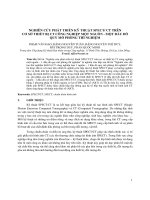
the mobile robot as shown in Fig. 2.1.

7


Fig. 2.1. Model of an Omni-directional mobile robot [47]
Dynamic equation of the robot as (2.1):
−a2d 0   xw   b1 1
 xw   a1
 y  = a 
a1
0   yw  + b1 3
 w  2 d
w   0
0
a3  w   b2
= AW β + BW U + D f

b1 2
b1 4
b2

2b1 cos    u1   D fx 


2b1 sin   u2  +  D fy 
b2   u3   D f  

(2.1)
where D f =  D fx

D fy

 a1

AW =  a2
 0


T

D f   are unknown system disturbances.

−a2
a1
0

0
 b1 1

0  ; BW = b1 3
 b2
a3 

U = u1

a2 = 1 − a2 =

u2

b1 2
b1 4
b2

2b1 cos  
2b1 sin   ;
b2 

u3 

T

3I w
;  1 = − 3 sin  − cos  ;  2 = 3 sin  − cos 
(3I w + 2Mr 2 )

 3 = 3 cos  − sin  ;  4 = − 3 cos  − sin 
2.4. Design of the sliding mode control law for the Omni-directional
mobile robot
2.4.1. Design of the sliding mode control law for the robot
Sliding mode controller is presented to ensure the actual trajectory of
the robot reaching a reference trajectory
Sliding mode control law is defined as (2.2) [108]:
8




(



)

U = − BW −1 AW  +  d + ke +  sign ( S )
−1
W

(2.2)

* Prove that the B matrix is invertible
We have:
b1 − 3 sin  − cos 

BW =  b1 3 cos  − sin 

b2


(
(

) b ( 3 sin  − cos )
) b ( − 3 cos  − sin  )
1

1

b2

determinant of BW as (2.4): det ( BW ) = 6 3b12b2  0
kr
krL
where: b1 =
; b2 =
2
(3I w + 2Mr )
(3I w + I v r 2 )

2b1 cos  

2b1 sin   (2.3)
b2 


(2.4)

Contains parameters of the robot such as the radius of the wheel (r);
the moment inertia of the wheel around the driving shaft (Iv); the mass of
the robot (M); Moment inertia of the wheel (Iw); Distance between any
assembly and the center gravity of the robot (L).
−1

This shows that the BW matrix is reversible and shows that the BW
matrix exists. Thus, there is a control rule (2.2) for robot.

Fig. 2.2. The structure of sliding mode control for robot

To prove the stability of the control law we need to prove that the
sliding mode surfaces converge to 0 according to Lyapunov. Lyapunov
function is defined as (2.5):

9


1 T
S S 0
2
Get the derivative of V, we have:
V = S T − AW  −  sign ( S )
V=

(

(

)

(2.5)

)

= − S T  +  sign ( S )  0

2.4.2. The parameters of the system and simulation results
Sliding mode controller is simulated to control an Omni-directional
mobile robot to ensure the following contents: (1) selection of a sliding
surface so as to achieve the desired system behavior, when the control

system reaches the sliding surface; and (2) selection of a control law such
that the existence of sliding mode can be guaranteed
The parameters of the system and controller are respectively given in
Table 2.1 and 2.2.
Table 2.1. The parameters of the mobile robot [47]
Notation

Meaning

Value

Unit

Iv

Moment inertia of
the mobile robot

11.25

kgm 2

M

Mass of the robot

9.4

kg

L

Distance between
any assembly and
the center gravity of
the robot

0.178

m

k

Driving gain factor

0.448

c

Viscous
friction
factor of the wheel

0.1889

kgm2 / s

I

Moment inertia of

the wheel

0.02108

kgm 2

r

Radius of the wheel

0.0245

m

10


Table 2.2. The parameters of the sliding mode control
Meaning

Sliding
parameters

Notation

Value

 x 0 0 



 0 y 0 
 0 0  



 20 0 0 
 0 20 0 


 0 0 20 

kx

0
0


 25 0 0 
 0 25 0 


 0 0 58 

0
ky
0

0

0

k 

➢ Case 1: the input is unit step function

Fig. 2.3. Responses xw , yw ,w

Fig. 2.4. Errors xw , yw ,w and

and xd , yd ,d with Step

xd , yd ,d with Step

Table 2.3. The quality criteria with unit step function
The quality criteria
Response
POT (%) exl (mm)
tqđ (s)
xw

0.20

0.22

0.45

yw

0.22

0.024

0.45

w

0.15

0.15

1.0

11


➢ Case 2: the input is unit step function when the mass of the robot
increases 25% and 50%

Fig. 2.5. Response xw when the

Fig. 2.6. Response yw when

mass of the robot increases

the mass of the robot

25% and 50%

increases 25% and 50%

➢ Case 3: the input is unit step function when the noise impacts at the

output

Fig. 2.7. Responses xw, yw and w

Fig. 2.8. Errors xw, yw và w when

when the noise impacts at the

the noise impacts at the output

output
The simulation results show that sliding mode controller has well
controlled robot converge to reach the reference trajectory. However, the
response of the SMC has yet to give optimal results with the achieved
quality criteria. To improve control quality, this study proposes using the
radial basic function neural network to estimate nonlinear function in
SMC law. The RBF is trained online by Gradient Descent algorithm and
12


considered as an adaptive controller due to the feedback from output
signals of the plant.
2.5. Design of the adaptive sliding mode control with neural networks
for the robot
2.5.1. The adaptive sliding mode control using RBF neural networks
In this part, the study uses Gradient Descent algorithm to estimate
online AW matrix in (2.2) SMC law. This matrix contains parameters of
the robot such as the radius of the wheel (r); the moment inertia of the
wheel around the driving shaft (Iv); the mass of the robot (M).
The algorithm of RBF neural network as (2.6) [41]:

 X −c
i
ij
hij = exp  −
2

2bij


2




 i =1,3; j =1,5

(2.6)

The general block diagram of the radial basis function neural network
is used to approximate the function fi in AW matrix is given in Fig. 2.9.

Fig. 2.9. Block diagram of the radial basis function neural network
where:

 X1   e (1) e (1)  d (1)

X i =  X 2  = e ( 2 ) e ( 2 )  d ( 2 )
 X 3   e ( 3) e ( 3)  d ( 3)
hij
=  hi1 hi 2 hi 3

i =1,2,3
13

 d (1)  d (1) 

d ( 2 ) d ( 2 )
 d ( 3)  d ( 3) 
hi 4

hi 5 

(2.7)
(2.8)


wij

i =1,2,3

=  wi1

wi 2

wi 3

wi 4

wi 5 

(2.9)

The output fi as (2.10): fi = wijT hij

(2.10)

The approximation matrix AW can be rewritten in the following form:
 w1jT h1j − w2jT d h2j
0 
 T

T
ˆ
(2.11)
AW =  w2j h2j
w1j h1j
0 
T
 0
0
w3j h3j 

Now, the adaptive sliding mode control using the RBF neural network
with Gradient Descent algorithm (GD-ASMC-RBF) is presented as (2.12):
(2.12)
U = − B −1 Aˆ  + (  + ke ) +  sign ( S )
W



W



d

When the actual trajectory of the robot deviates from the reference
trajectory due to the impact of actual conditions such as road surface
friction, changing inertial torque, .... the error changes. At that time, the
RBF network will be automatically updated with Gradient Descent
algorithm, which AˆW will also change so that the error reaches the
minimum value. We say the control law (2.12) adapts to the robot's
operating conditions
To prove the stability of the control law we need to prove that the
sliding mode surfaces converge to 0 according to Lyapunov. Lyapunov
function is defined as (2.13):

1 T
S S 0
2
Get the derivative of V, we have:
V = S T − AˆW  −  sign ( S ) = S T − −  sign ( S )
V=

(

)

(

(

(2.13)

)

)

= − S T  +  sign ( S )  0

2.5.2. The parameters of the system and simulation results
- Sliding mode controller is defined to guarantee state trajectory not
only converges to the sliding surface in finite time but also remains on the
sliding surface even when the system parameters are changed.
14


- The Gradient Descent algorithm effects in online approximation of
nonlinear matrix of the SMC law.
- The adaptive sliding mode control is stable when the actual
trajectory of the robot deviates from the reference trajectory due to the
impact of actual conditions or by changing the parameters of the plant.
The parameters of the radial basis function neural network are shown
in Table 2.4:
Table 2.4. The parameters of the radial basis function neural network
Notation

Meaning

Value



Momentum factor

0.05



Learning factor

0.5

0.5 0.5

cij

Center vector for the neural
network

 −1
 −1

 −1

 −1
 −1

−0.5 0 0.5 1
−0.5 0 0.5 1
−0.5 0 0.5 1


−0.5 0 0.5 1
−0.5 0 0.5 1

bj

Certain threshold of the
neural network

1

Parameter vector

0.5 0.5 0.5 0.5 0.5
0.5 0.5 0.5 0.5 0.5


0.5 0.5 0.5 0.5 0.5

W 
V 
 
 Z 

T

1 1 1 1

T

i

Total inputs

5

j

Total neurons in hidden
layers

5

15


➢ Case 1: the input is unit step function

Fig. 2.10. Responses GD-

Fig. 2.11. Errors GD-ASMC-

ASMC-RBF and SMC

RBF and SMC controller with

controller with Step

Step

Table 2.5. The quality criteria of the GD-ASMC-RBF controller with
unit step function
Response

The quality criteria
POT (%)

exl (mm)

tqđ (s)

xw

0.15

0

0.3

yw

0.62

0.55

0.3

w

0.80

0

0.4

Table 2.6. The error performances between GD-ASMC-RBF and SMC
Response

SMC

GD-ASMC-RBF

ADD

MSE

RMSE

ADD

MSE

RMSE

xw

1.4×10-4

3.9×10-8

2.0×10-4

4.9×10-5

4.9×10-9

7.0×10-5

yw

1.1×10-4

2.5×10-8

1.6×10-4

8.6×10-5

1.5×10-8

1.2×10-4

w

2.3×10-5

1.1×10-9

3.3×10-5

4.2×10-5

3.6×10-9

6.0×10-5

16


➢ Case 2: the input is unit step function when the noise impacts at the
output

Fig. 2.12. Responses of the

Fig. 2.13. Errors of the GD-

GD-ASMC-RBF and SMC

ASMC-RBF and SMC with

with unit step function

unit step function when the

when the noise impacts at

noise impacts at the output

the output
The simulation results of the GD-ASMC-RBF controller for Omnidirectional mobile robot have good results, the response of the robot

converge to reach the trajectory without steady-state error even
disturbances of the system. This is the remarkable feature of the sliding
mode controller as well as the Gradient Descent algorithm in the online
approximation of the Aw matrix in SMC law. This shows the feasibility of
GD-ASMC-RBF controller in nonlinear system control

17


CHAPTER 3: EVALUATING THE EFFECTIVENESS OF THE
QUASI-NEWTON ALGORITHM IN NONLINEAR SYSTEM
TRAJECTORY TRACKING CONTROL
3.1. Problem
In chapter 2, the author is used the RBF neural network to estimate
nonlinear functions in the sliding mode control law which is calculated
based on Lyapunov stability theory of adaptive sliding mode controller
based on RBF neural network. The simulation results with
MATLAB/SIMULINK show that the proposed algorithm is efficient, the
response of the robot converge to reach the trajectory without steady-state
error is about, and the rise time is about 0.3 ± 0.001(s) . However,
Gradient Descent algorithm is limited such as: slow convergence speed,
easy to fall into the local minimum and the ability to search the whole
world inefficient [22, 37]. In this chapter 3, research proposes using a
Quasi-Newton algorithm to train online the RBF neural network, at the
same time the research investigates the influence of the parameters of
neural network (number of hidden) on the control quality of the adaptive
sliding mode control.
3.2. The object
- The RBF neural networks are trained online using Quasi-Newton
algorithm with initial parameters are randomly generated

- The proposed algorithm is applied in Omni-directional mobile robot
trajectory tracking control.
- the research investigates the influence of number of hidden layers on
the control quality of an adaptive sliding mode control using radial basis
function neural networks.
3.3. Evaluate the performance of the Quasi-Newton algorithm in
nonlinear system trajectory tracking control
18


3.3.1. The Quasi-Newton algorithm
This algorithm onsists of 4 steps with k iteration
Step 1: Initialize search direction by (3.1)

d k = − H k−1 gk .

(3.1)

Step 2 : Search in the direction d k to find the step length  k .
f ( wk +  k d k ) = min ( f ( wk +  k d k ) ) .
 0

E ( wk +  k d k )  E ( wk ) +  k gkT d k
g ( wk +  k d k )  − gkT d k
T

(3.2)

The weight update process is presented as (3.3).

wk +1 = wk +  k d k

(3.3)

Step 3 : The Hessian matrix update process is presented as (3.4).
g g T H   T H
(3.4)
H k +1 = H k + k T k − k T k k k
gk  k
 k H k k
Step 4 : heck convergence with some standards. Typically, this
standard is defined as a direction of the objective function to ensure that
it is less than a given value to stop iteration as (3.5)

gkT gk   .

(3.5)

The iteration begins when k = 0 , the initialization process is random,
the Hessian matrix H 0 is a symmetric matrix and is a positive
determination matrix with initial value H 0 = I .
3.3.2. Training online the RBF neural network by the Quasi-Newton
algorithm applied in the adaptive sliding mode control Omni-directional
mobile robot.
In this part, the study uses the Quasi-Newton algorithm to approximate

AW matrix in SMC law (2.2) instead of Gradient Descent.
The algorithm of the RBF neural network as (2.6).
The RBF neural network’s structure is used to approximate the fi
component in AW matrix as Fig. 2.9 in Chapter 2.

19


Where Xi and hij as (2.7) and (2.8).
And t ij i =1,2,3 = ti1 ti 2 ti 3 ti 4 ti 5 

(3.6)

The output fi as (3.7): fi = tijT hij
(3.7)
Hence, the approximation matrix AW can be rewritten as (3.8):
 t1jT h1j −t 2jT d h2j
0 
T

T
ˆ
(3.8)
AW =  t 2j h2j
t1j h1j
0 
T
 0
0
t3j h3j 

The adaptive sliding mode control law using the RBF neural network
which is trained online by the Quasi-Newton algorithm (QN-ASMCRBF) as (3.9):



(

)



U = − BW −1 AˆW  +  d + ke +  sign ( S )

(3.9)

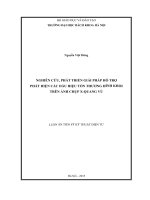
The result of online training of RBF neural network with QuasiNewton algorithm (BSGS) presented as Fig. 3.1 with MSE (Mean Square
Error) are smaller than Gradient Descent algorithm. This has great
significance in improving controller response, especially in controller
online training

Fig. 3.1. Compare MSE of Quasi-Newton (BSGS) and Gradient
Descent

20


The simulation diagram of the QN-ASMC-RBF in MATLAB
/SIMULINK to control Omni-directional mobile robot with simulation
parameters of the robot still used as in Chapter 2.
➢ Case 1: the input is unit step function

Fig. 3.2. Reponses xw, yw and w

Fig. 3.3. Errors xw, yw and w of

of the QN-ASMC-RBF with

the QN-ASMC-RBF with Step

Step
Table 3.1. The quality criteria of the QN-ASMC-RBF with Step
Reponses

QN-ASMC-RBF
POT (%)

exl (mm)

tqđ (s)

xw

0

1.5

0.2

yw

0.19

0

0.2

w

0.05

0

0.18

Table 3.2. The error performances between GD-ASMC-RBF and QNASMC-RBF
Reponses

QN-ASMC-RBF

GD-ASMC-RBF

ADD

MSE

RMSE

ADD

MSE

RMSE

xw

9.8×10-4

1.9×10-6

0.0014

2.2×10-4

9.4×10-8

3.0×10-4

yw

7.1×10-4

1.0×10-6

1.0×10-3

2.6×10-4

1.5×10-7

3.7×10-4

w

2.0×10-5

8.3×10-10

2.9×10-5

9.2×10-5

1.6×10-8

1.3×10-4

21


➢ Case 2: the input is unit step function when the noise impacts at the
output

Fig. 3.4. Reponses xw, yw

Fig. 3.5. Errors xw, yw and

and w of the QN-ASMC-

w of the QN-ASMC-RBF

RBF with Step when the

with Step when the noise

noise impacts at the output

impacts at the output

The advantage of this controller is the convergence speed of BFGS
method is faster than Gradient Descent method; the quality criteria of the
adaptive sliding control with neural network are trained online by QuasiNewton algorithm with BFGS smaller than Gradient Descent algorithm
in the same network structure; control rules adapts according to the
operating conditions of the robot. However, the parameters of neural
networks, such as the number of hidden layers, thresholds and
initialization weights are randomly selected. This problem will be solved
in Chapter 4 to ensure the network structure is optimal.
3.3.3. Investigate the influence of the RBF neural networks parameters
on the control quality of the adaptive sliding mode control
The author investigates the influence of the neural networks structure
on the control quality of the adaptive sliding mode control with the
number of hidden layers is 1, 3, 5, 7, 9, 11, 13, 15, 17 and 19. The weight
update result and the performances of this algorithm are presented in
Table 3.4 and 3.5.
22


CHAPTER 4: OPTIMIZING THE STRUCTURE OF NEURAL
NETWORK USING GENETIC ALGORITHM
4.1. Introduction
In this Chapter 4, the study optimizes the structure and the parameters
of the RBF neural network by genetic algorithm. First, genetic algorithm
is used to determine the number of neurons in the hidden layer of the RBF
neural network; then this result is used to find the best values of the
centers, widths and initial weights. After optimizing, the radial basis
function neural network is online trained by Quasi - Newton algorithm in

trajectory tracking control of the omni-directional mobile robot
4.2. Optimize the structure and the parameters of the neural network
using genetic algorithm
The overall diagram of the optimizing the structure and the parameters
of neural networks using genetic algorithm is shown in Fig. 4.1:

Fig. 4.1. Diagram of GA-ASMC-RBF Control
Parameters for the complete GA algorithm are shown in Table 4.1
➢ Using the network training error and the number of hidden neurons
to determine the RBF neural networks’ corresponding fitness of the
chromosomes. Suppose the training error is 𝐸, the number of neurons in
the hidden layer is 𝑠, and upper limit of the number of neurons in the
hidden layer is 𝑠max.
23


- Condition:

 s  smax

−6
2
 E  25  10 (m )

(4.1)

- The fitness 𝐹 of GA is defined by (4.7) [90, 104]:
s
F =C−E
( m)

smax

(4.2)

where, C (m2) is a constant selected through experimentation, smax is
the maximum number of neurons in the hidden layer, we choose smax = 50.
➢ In each generation of GA, we use the formula (4.3) as the target
function for the Quasi-Newtonian algorithm to update the parameters of
neural networks [75, 104].

1
(4.3)
E = ( d −  w )2
2
Where, E is the Mean Square Error, βd is the desired input signal and
βw is the output of the object.
Table 4.1. Parameters of the GA algorithm
Optimal structure

Optimal parameters

the RBF network

the RBF network

Generation number

15

15

Population size

20

30

0.7

0.7

0.01 – 0.001

0.01 – 0.001

Parameters

Frequency

of

hybridization
Probability

of

mutation
Selective
Objective function

Roulette
s
F =C−E
smax

24

Roulette

1
E = ( d −  w )2
2


The results of the RBF neural network using GA are shown in Fig. 4.2
và 4.3.

Fig. 4.2. Diagram indicate the

Fig. 4.3. Diagram indicate the

value of the objective function in

value of the objective function in

structure optimal RBF network.

weights optimal RBF network.

The number of hidden layer neurons and parameters of RBF neurons

after optimization by genetic algorithms are presented in Table 4.2.
Table 4.2. Structure and parameters of the RBF network using the GA
algorithm
Notation

Value

b

10.6022
1.76 −11.01
 12.41 −0.47 −1.73 −12.08 9.89
 −4.39 1.19 −13.67 −2.88
9.83 10.35 −13.91

 −1.65 12.30
7.07
−9.59
3.02 −3.92 −12.82 


 6.25 5.15 −2.06 −2.69 −10.11 −2.20 3.98 
13.58 4.00 −0.88 −3.90 −1.98 4.42 −1.46 
4.81 0.77 −1.24 0.90 −1.78 1.58 −2.41

cij

T1

T2

T3

−3.92 0.87
3.57 −2.82

−1.86 −1.48 −2.24 −2.00 −2.45

2.38 −1.16 −4.50 4.18 1.77

j

7

From Table 4.2, it is observed that the genetic algorithm has
determined the specific values of the hidden layer neuron, center,
25