Giáo trình principles of communications systems modulation and noise 7e by ziểm tranter
Bạn đang xem bản rút gọn của tài liệu. Xem và tải ngay bản đầy đủ của tài liệu tại đây (16.82 MB, 746 trang )
PRINCIPLES OF
COMMUNICATIONS
Systems, Modulation,
and Noise
SEVENTH EDITION
RODGER E. ZIEMER
University of Colorado at Colorado Springs
WILLIAM H. TRANTER
Virginia Polytechnic Institute and State University
VP & PUBLISHER:
EXECUTIVE EDITOR:
SPONSORING EDITOR:
PROJECT EDITOR:
COVER DESIGNER:
ASSOCIATE PRODUCTION MANAGER:
SENIOR PRODUCTION EDITOR:
PRODUCTION MANAGEMENT SERVICES:
COVER ILLUSTRATION CREDITS:
Don Fowley
Dan Sayre
Mary O’Sullivan
Ellen Keohane
Kenji Ngieng
Joyce Poh
Jolene Ling
Thomson Digital
© Rodger E. Ziemer, William H. Tranter
This book was set by Thomson Digital.
Founded in 1807, John Wiley & Sons, Inc. has been a valued source of knowledge and understanding for more than
200 years, helping people around the world meet their needs and fulfill their aspirations. Our company is built on a
foundation of principles that include responsibility to the communities we serve and where we live and work. In
2008, we launched a Corporate Citizenship Initiative, a global effort to address the environmental, social, economic,
and ethical challenges we face in our business. Among the issues we are addressing are carbon impact, paper
specifications and procurement, ethical conduct within our business and among our vendors, and community and
charitable support. For more information, please visit our website: www.wiley.com/go/citizenship.
Copyright © 2015, 2009, 2002, 1995 John Wiley & Sons, Inc. All rights reserved. No part of this publication may be
reproduced, stored in a retrieval system or transmitted in any form or by any means, electronic, mechanical,
photocopying, recording, scanning or otherwise, except as permitted under Sections 107 or 108 of the 1976 United
States Copyright Act, without either the prior written permission of the Publisher, or authorization through payment
of the appropriate per-copy fee to the Copyright Clearance Center, Inc. 222 Rosewood Drive, Danvers, MA 01923,
website www.copyright.com. Requests to the Publisher for permission should be addressed to the Permissions
Department, John Wiley & Sons, Inc., 111 River Street, Hoboken, NJ 07030-5774, (201)748-6011,
fax (201)748-6008, website />Evaluation copies are provided to qualified academics and professionals for review purposes only, for use in their
courses during the next academic year. These copies are licensed and may not be sold or transferred to a third party.
Upon completion of the review period, please return the evaluation copy to Wiley. Return instructions and a free of
charge return mailing label are available at www.wiley.com/go/returnlabel. If you have chosen to adopt this
textbook for use in your course, please accept this book as your complimentary desk copy. Outside of the United
States, please contact your local sales representative.
Library of Congress Cataloging-in-Publication Data:
Ziemer, Rodger E.
Principles of communication : systems, modulation, and noise / Rodger E. Ziemer,
William H. Tranter. − Seventh edition.
pages cm
Includes bibliographical references and index.
ISBN 978-1-118-07891-4 (paper)
1. Telecommunication. 2. Signal theory (Telecommunication) I. Tranter,
William H. II. Title.
TK5105.Z54 2014
621.382’2−dc23
2013034294
Printed in the United States of America
10
9
8
7
6
5
4
3
2
1
PREFACE
The first edition of this book was published in 1976, less than a decade after Neil Armstrong became the
first man to walk on the moon in 1969. The programs that lead to the first moon landing gave birth to
many advances in science and technology. A number of these advances, especially those in microelectronics
and digital signal processing (DSP), became enabling technologies for advances in communications. For
example, prior to 1969, essentially all commercial communication systems, including radio, telephones, and
television, were analog. Enabling technologies gave rise to the internet and the World Wide Web, digital radio
and television, satellite communications, Global Positioning Systems, cellular communications for voice and
data, and a host of other applications that impact our daily lives. A number of books have been written that
provide an in-depth study of these applications. In this book we have chosen not to cover application areas in
detail but, rather, to focus on basic theory and fundamental techniques. A firm understanding of basic theory
prepares the student to pursue study of higher-level theoretical concepts and applications.
True to this philosophy, we continue to resist the temptation to include a variety of new applications
and technologies in this edition and believe that application examples and specific technologies, which often
have short lifetimes, are best treated in subsequent courses after students have mastered the basic theory and
analysis techniques. Reactions to previous editions have shown that emphasizing fundamentals, as opposed
to specific technologies, serve the user well while keeping the length of the book reasonable. This strategy
appears to have worked well for advanced undergraduates, for new graduate students who may have forgotten
some of the fundamentals, and for the working engineer who may use the book as a reference or who may
be taking a course after-hours. New developments that appear to be fundamental, such as multiple-input
multiple-output (MIMO) systems and capacity-approaching codes, are covered in appropriate detail.
The two most obvious changes to the seventh edition of this book are the addition of drill problems to
the Problems section at the end of each chapter and the division of chapter three into two chapters. The drill
problems provide the student problem-solving practice with relatively simple problems. While the solutions
to these problems are straightforward, the complete set of drill problems covers the important concepts of
each chapter. Chapter 3, as it appeared in previous editions, is now divided into two chapters mainly due to
length. Chapter 3 now focuses on linear analog modulation and simple discrete-time modulation techniques
that are direct applications of the sampling theorem. Chapter 4 now focuses on nonlinear modulation
techniques. A number of new or revised end-of-chapter problems are included in all chapters.
In addition to these obvious changes, a number of other changes have been made in edition seven. An
example on signal space was deleted from Chapter 2 since it is really not necessary at this point in the book.
(Chapter 11 deals more fully with the concepts of signal space.) Chapter 3, as described in the previous
paragraph, now deals with linear analog modulation techniques. A section on measuring the modulation index
of AM signals and measuring transmitter linearity has been added. The section on analog television has been
deleted from Chapter 3 since it is no longer relevant. Finally, the section on adaptive delta modulation has
been deleted. Chapter 4 now deals with non-linear analog modulation techniques. Except for the problems,
no significant additions or deletions have been made to Chapter 5. The same is true of Chapters 6 and 7,
which treat probability and random processes, respectively. A section on signal-to-noise ratio measurement
has been added to Chapter 8, which treats noise effects in modulation systems. More detail on basic channel
iii
iv
Preface
models for fading channels has been added in Chapter 9 along with simulation results for bit error rate (BER)
performance of a minimum mean-square error (MMSE) equalizer with optimum weights and an additional
example of the MMSE equalizer with adaptive weights. Several changes have been made to Chapter 10.
Satellite communications was reluctantly deleted because it would have required adding several additional
pages to do it justice. A section was added on MIMO systems using the Alamouti approach, which concludes
with a BER curve comparing performances of 2-transmit 1-receive Alamouti signaling in a Rayleigh fading
channel with a 2-transmit 2-receive diversity system. A short discussion was also added to Chapter 10
illustrating the features of 4G cellular communications as compared with 2G and 3G systems. With the
exception of the Problems, no changes have been made to Chapter 11. A ‘‘Quick Overview’’ section has
been added to Chapter 12 discussing capacity-approaching codes, run-length codes, and digital television.
A feature of the later editions of Principles of Communications was the inclusion of several computer
examples within each chapter. (MATLAB was chosen for these examples because of its widespread use
in both academic and industrial settings, as well as for MATLAB’s rich graphics library.) These computer
examples, which range from programs for computing performance curves to simulation programs for certain
types of communication systems and algorithms, allow the student to observe the behavior of more complex
systems without the need for extensive computations. These examples also expose the student to modern
computational tools for analysis and simulation in the context of communication systems. Even though we
have limited the amount of this material in order to ensure that the character of the book is not changed,
the number of computer examples has been increased for the seventh edition. In addition to the in-chapter
computer examples, a number of ‘‘computer exercises’’ are included at the end of each chapter. The number
of these has also been increased in the seventh edition. These exercises follow the end-of-chapter problems
and are designed to make use of the computer in order to illustrate basic principles and to provide the student
with additional insight. A number of new problems have been included at the end of each chapter in addition
to a number of problems that were revised from the previous edition.
The publisher maintains a web site from which the source code for all in-chapter computer examples
can be downloaded. Also included on the web site are Appendix G (answers to the drill problems) and the
bibliography. The URL is
www.wiley.com/college/ziemer
We recommend that, although MATLAB code is included in the text, students download MATLAB code
of interest from the publisher website. The code in the text is subject to printing and other types of errors and
is included to give the student insight into the computational techniques used for the illustrative examples.
In addition, the MATLAB code on the publisher website is periodically updated as need justifies. This web
site also contains complete solutions for the end-of-chapter problems and computer exercises. (The solutions
manual is password protected and is intended only for course instructors.)
We wish to thank the many persons who have contributed to the development of this textbook and
who have suggested improvements for this and previous editions of this book. We also express our thanks
to the many colleagues who have offered suggestions to us by correspondence or verbally as well as the
industries and agencies that have supported our research. We especially thank our colleagues and students
at the University of Colorado at Colorado Springs, the Missouri University of Science and Technology, and
Virginia Tech for their comments and suggestions. It is to our students that we dedicate this book. We have
worked with many people over the past forty years and many of them have helped shape our teaching and
research philosophy. We thank them all.
Finally, our families deserve much more than a simple thanks for the patience and support that they have
given us throughout forty years of seemingly endless writing projects.
Rodger E. Ziemer
William H. Tranter
CONTENTS
CHAPTER
1
INTRODUCTION
1.1
1.2
2.4.4
2.4.5
1
4
The Block Diagram of a Communication System
Channel Characteristics 5
1.2.1
1.2.2
Noise Sources 5
Types of Transmission Channels
7
Summary of Systems-Analysis Techniques 13
1.3.1 Time and Frequency-Domain Analyses 13
1.3.2 Modulation and Communication Theories 13
1.4 Probabilistic Approaches to System Optimization 14
1.4.1 Statistical Signal Detection and Estimation
Theory 14
1.4.2 Information Theory and Coding 15
1.4.3 Recent Advances 16
1.5 Preview of This Book 16
Further Reading 16
1.3
CHAPTER
2
SIGNAL AND LINEAR SYSTEM ANALYSIS 17
2.1
2.2
2.3
2.4
Signal Models
17
2.1.1 Deterministic and Random Signals 17
2.1.2 Periodic and Aperiodic Signals 18
2.1.3 Phasor Signals and Spectra 18
2.1.4 Singularity Functions 21
Signal Classifications 24
Fourier Series 26
2.3.1 Complex Exponential Fourier Series 26
2.3.2 Symmetry Properties of the Fourier
Coefficients 27
2.3.3 Trigonometric Form of the Fourier Series
2.3.4 Parseval’s Theorem 28
2.3.5 Examples of Fourier Series 29
2.3.6 Line Spectra 30
The Fourier Transform 34
2.4.1 Amplitude and Phase Spectra
2.4.2 Symmetry Properties 36
2.4.3 Energy Spectral Density 37
35
28
2.4.6
2.4.7
Convolution 38
Transform Theorems: Proofs and
Applications 40
Fourier Transforms of Periodic Signals
Poisson Sum Formula 50
48
2.5 Power Spectral Density and Correlation 50
2.5.1 The Time-Average Autocorrelation Function
2.5.2 Properties of 𝑅(𝜏) 52
2.6 Signals and Linear Systems 55
51
2.6.1
Definition of a Linear Time-Invariant
System 56
2.6.2 Impulse Response and the Superposition
Integral 56
2.6.3 Stability 58
2.6.4 Transfer (Frequency Response) Function 58
2.6.5 Causality 58
2.6.6 Symmetry Properties of 𝐻(𝑓 ) 59
2.6.7 Input-Output Relationships for Spectral
Densities 62
2.6.8 Response to Periodic Inputs 62
2.6.9 Distortionless Transmission 64
2.6.10 Group and Phase Delay 64
2.6.11 Nonlinear Distortion 67
2.6.12 Ideal Filters 68
2.6.13 Approximation of Ideal Lowpass Filters by
Realizable Filters 70
2.6.14 Relationship of Pulse Resolution and Risetime to
Bandwidth 75
2.7 Sampling Theory 78
2.8 The Hilbert Transform 82
2.8.1 Definition 82
2.8.2 Properties 83
2.8.3 Analytic Signals 85
2.8.4 Complex Envelope Representation of Bandpass
Signals 87
2.8.5 Complex Envelope Representation of Bandpass
Systems 89
2.9 The Discrete Fourier Transform and Fast Fourier
Transform 91
Further Reading 95
v
vi
Contents
Summary 95
Drill Problems 98
Problems 100
Computer Exercises
CHAPTER
4.5 Analog Pulse Modulation
4.5.1
4.5.2
111
3
LINEAR MODULATION TECHNIQUES
3.1
3.2
3.3
3.4
3.5
3.6
3.7
3.8
4.6 Multiplexing 204
4.6.1 Frequency-Division Multiplexing 204
4.6.2 Example of FDM: Stereophonic FM
Broadcasting 205
4.6.3 Quadrature Multiplexing 206
4.6.4 Comparison of Multiplexing Schemes 207
Further Reading 208
Summary 208
Drill Problems 209
Problems 210
Computer Exercises 213
112
Double-Sideband Modulation 113
Amplitude Modulation (AM) 116
3.2.1
3.2.2
Envelope Detection 118
The Modulation Trapezoid
122
Single-Sideband (SSB) Modulation 124
Vestigial-Sideband (VSB) Modulation 133
Frequency Translation and Mixing 136
Interference in Linear Modulation 139
Pulse Amplitude Modulation---PAM 142
Digital Pulse Modulation 144
3.8.1 Delta Modulation 144
3.8.2 Pulse-Code Modulation 146
3.8.3 Time-Division Multiplexing 147
3.8.4 An Example: The Digital Telephone System
CHAPTER
149
4
ANGLE MODULATION AND
MULTIPLEXING 156
4.1
4.2
4.3
4.4
Phase and Frequency Modulation Defined 156
4.1.1 Narrowband Angle Modulation 157
4.1.2 Spectrum of an Angle-Modulated Signal 161
4.1.3 Power in an Angle-Modulated Signal 168
4.1.4 Bandwidth of Angle-Modulated Signals 168
4.1.5 Narrowband-to-Wideband Conversion 173
Demodulation of Angle-Modulated Signals 175
Feedback Demodulators: The Phase-Locked
Loop 181
4.3.1 Phase-Locked Loops for FM and PM
Demodulation 181
4.3.2 Phase-Locked Loop Operation in the Tracking
Mode: The Linear Model 184
4.3.3 Phase-Locked Loop Operation in the Acquisition
Mode 189
4.3.4 Costas PLLs 194
4.3.5 Frequency Multiplication and Frequency
Division 195
Interference in Angle Modulation
196
5
PRINCIPLES OF BASEBAND DIGITAL DATA
TRANSMISSION 215
Further Reading 150
Summary 150
Drill Problems 151
Problems 152
Computer Exercises 155
CHAPTER
201
Pulse-Width Modulation (PWM) 201
Pulse-Position Modulation (PPM) 203
5.1 Baseband Digital Data Transmission Systems 215
5.2 Line Codes and Their Power Spectra 216
5.2.1 Description of Line Codes 216
5.2.2 Power Spectra for Line-Coded Data 218
5.3 Effects of Filtering of Digital Data---ISI 225
5.4 Pulse Shaping: Nyquist’s Criterion for Zero ISI 227
5.4.1 Pulses Having the Zero ISI Property 228
5.4.2 Nyquist’s Pulse-Shaping Criterion 229
5.4.3 Transmitter and Receiver Filters for
Zero ISI 231
5.5 Zero-Forcing Equalization 233
5.6 Eye Diagrams 237
5.7 Synchronization 239
5.8 Carrier Modulation of Baseband Digital Signals
Further Reading 244
Summary 244
Drill Problems 245
Problems 246
Computer Exercises 249
CHAPTER
6
OVERVIEW OF PROBABILITY AND RANDOM
VARIABLES 250
6.1 What is Probability?
6.1.1
6.1.2
6.1.3
6.1.4
6.1.5
250
Equally Likely Outcomes 250
Relative Frequency 251
Sample Spaces and the Axioms of
Probability 252
Venn Diagrams 253
Some Useful Probability Relationships
253
243
Contents
6.2
6.1.6 Tree Diagrams 257
6.1.7 Some More General Relationships 259
Random Variables and Related Functions 260
6.2.1
6.2.2
Random Variables 260
Probability (Cumulative) Distribution
Functions 262
6.2.3 Probability-Density Function 263
6.2.4 Joint cdfs and pdfs 265
6.2.5 Transformation of Random Variables 270
Statistical Averages 274
6.3.1 Average of a Discrete Random Variable 274
6.3.2 Average of a Continuous Random Variable 275
6.3.3 Average of a Function of a Random
Variable 275
6.3.4 Average of a Function of More Than One
Random Variable 277
6.3.5 Variance of a Random Variable 279
6.3.6 Average of a Linear Combination of 𝑁 Random
Variables 280
6.3.7 Variance of a Linear Combination of Independent
Random Variables 281
6.3.8 Another Special Average---The Characteristic
Function 282
6.3.9 The pdf of the Sum of Two Independent Random
Variables 283
6.3.10 Covariance and the Correlation Coefficient 285
6.4 Some Useful pdfs 286
6.4.1 Binomial Distribution 286
6.4.2 Laplace Approximation to the Binomial
Distribution 288
6.4.3 Poisson Distribution and Poisson Approximation
to the Binomial Distribution 289
6.4.4 Geometric Distribution 290
6.4.5 Gaussian Distribution 291
6.4.6 Gaussian 𝑄-Function 295
6.4.7 Chebyshev’s Inequality 296
6.4.8 Collection of Probability Functions and Their
Means and Variances 296
Further Reading 298
Summary 298
Drill Problems 300
Problems 301
Computer Exercises 307
6.3
CHAPTER
7
RANDOM SIGNALS AND NOISE 308
7.1
7.2
A Relative-Frequency Description of Random
Processes 308
Some Terminology of Random Processes 310
7.2.1 Sample Functions and Ensembles 310
7.2.2
7.2.3
7.2.4
7.2.5
vii
Description of Random Processes in Terms of
Joint pdfs 311
Stationarity 311
Partial Description of Random Processes:
Ergodicity 312
Meanings of Various Averages for Ergodic
Processes 315
7.3 Correlation and Power Spectral Density 316
7.3.1 Power Spectral Density 316
7.3.2 The Wiener--Khinchine Theorem 318
7.3.3 Properties of the Autocorrelation Function 320
7.3.4 Autocorrelation Functions for Random Pulse
Trains 321
7.3.5 Cross-Correlation Function and Cross-Power
Spectral Density 324
7.4 Linear Systems and Random Processes 325
7.4.1 Input-Output Relationships 325
7.4.2 Filtered Gaussian Processes 327
7.4.3 Noise-Equivalent Bandwidth 329
7.5 Narrowband Noise 333
7.5.1 Quadrature-Component and Envelope-Phase
Representation 333
7.5.2 The Power Spectral Density Function of 𝑛𝑐 (𝑡) and
𝑛𝑠 (𝑡) 335
7.5.3 Ricean Probability Density Function 338
Further Reading 340
Summary 340
Drill Problems 341
Problems 342
Computer Exercises 348
CHAPTER
8
NOISE IN MODULATION SYSTEMS 349
8.1 Signal-to-Noise Ratios 350
8.1.1 Baseband Systems 350
8.1.2 Double-Sideband Systems 351
8.1.3 Single-Sideband Systems 353
8.1.4 Amplitude Modulation Systems 355
8.1.5 An Estimator for Signal-to-Noise Ratios 361
8.2 Noise and Phase Errors in Coherent Systems 366
8.3 Noise in Angle Modulation 370
8.3.1 The Effect of Noise on the Receiver Input 370
8.3.2 Demodulation of PM 371
8.3.3 Demodulation of FM: Above Threshold
Operation 372
8.3.4 Performance Enhancement through the Use of
De-emphasis 374
8.4 Threshold Effect in FM Demodulation 376
8.4.1
Threshold Effects in FM Demodulators
376
viii
8.5
Contents
Noise in Pulse-Code Modulation
384
8.5.1 Postdetection SNR 384
8.5.2 Companding 387
Further Reading 389
Summary 389
Drill Problems 391
Problems 391
Computer Exercises 394
CHAPTER
9
PRINCIPLES OF DIGITAL DATA TRANSMISSION
IN NOISE 396
9.1
9.2
Baseband Data Transmission in White Gaussian
Noise 398
Binary Synchronous Data Transmission with
Arbitrary Signal Shapes 404
9.2.1
9.2.2
9.2.3
9.3
9.4
9.5
9.6
9.7
9.8
9.9
Receiver Structure and Error Probability 404
The Matched Filter 407
Error Probability for the Matched-Filter
Receiver 410
9.2.4 Correlator Implementation of the Matched-Filter
Receiver 413
9.2.5 Optimum Threshold 414
9.2.6 Nonwhite (Colored) Noise Backgrounds 414
9.2.7 Receiver Implementation Imperfections 415
9.2.8 Error Probabilities for Coherent Binary
Signaling 415
Modulation Schemes not Requiring Coherent
References 421
9.3.1 Differential Phase-Shift Keying (DPSK) 422
9.3.2 Differential Encoding and Decoding of Data 427
9.3.3 Noncoherent FSK 429
M-ary Pulse-Amplitude Modulation (PAM) 431
Comparison of Digital Modulation Systems 435
Noise Performance of Zero-ISI Digital Data
Transmission Systems 438
Multipath Interference 443
Fading Channels 449
9.8.1 Basic Channel Models 449
9.8.2 Flat-Fading Channel Statistics and Error
Probabilities 450
Equalization 455
9.9.1 Equalization by Zero-Forcing 455
9.9.2 Equalization by MMSE 459
9.9.3 Tap Weight Adjustment 463
Further Reading 466
Summary 466
Drill Problems 468
Problems 469
Computer Exercises 476
CHAPTER
10
ADVANCED DATA COMMUNICATIONS
TOPICS 477
10.1 M-ary Data Communications Systems 477
10.1.1 M-ary Schemes Based on Quadrature
Multiplexing 477
10.1.2 OQPSK Systems 481
10.1.3 MSK Systems 482
10.1.4 M-ary Data Transmission in Terms of Signal
Space 489
10.1.5 QPSK in Terms of Signal Space 491
10.1.6 M-ary Phase-Shift Keying 493
10.1.7 Quadrature-Amplitude Modulation
(QAM) 495
10.1.8 Coherent FSK 497
10.1.9 Noncoherent FSK 498
10.1.10 Differentially Coherent Phase-Shift
Keying 502
10.1.11 Bit Error Probability from Symbol Error
Probability 503
10.1.12 Comparison of M-ary Communications Systems
on the Basis of Bit Error Probability 505
10.1.13 Comparison of M-ary Communications Systems
on the Basis of Bandwidth Efficiency 508
10.2 Power Spectra for Digital Modulation 510
10.2.1 Quadrature Modulation Techniques 510
10.2.2 FSK Modulation 514
10.2.3 Summary 516
10.3 Synchronization 516
10.3.1 Carrier Synchronization 517
10.3.2 Symbol Synchronization 520
10.3.3 Word Synchronization 521
10.3.4 Pseudo-Noise (PN) Sequences 524
10.4 Spread-Spectrum Communication Systems 528
10.4.1 Direct-Sequence Spread Spectrum 530
10.4.2 Performance of DSSS in CW Interference
Environments 532
10.4.3 Performance of Spread Spectrum in Multiple
User Environments 533
10.4.4 Frequency-Hop Spread Spectrum 536
10.4.5 Code Synchronization 537
10.4.6 Conclusion 539
10.5 Multicarrier Modulation and Orthogonal
Frequency-Division Multiplexing 540
10.6 Cellular Radio Communication Systems 545
10.6.1 Basic Principles of Cellular Radio 546
10.6.2 Channel Perturbations in Cellular Radio 550
10.6.3 Multiple-Input Multiple-Output (MIMO)
Systems---Protection Against Fading 551
10.6.4 Characteristics of 1G and 2G Cellular
Systems 553
Contents
10.6.5 Characteristics of cdma2000 and
W-CDMA 553
10.6.6 Migration to 4G 555
Further Reading 556
Summary 556
Drill Problems 557
Problems 558
Computer Exercises 563
11.5.2 Estimation of Signal Phase: The PLL
Revisited 604
Further Reading 606
Summary 607
Drill Problems 607
Problems 608
Computer Exercises 614
CHAPTER
CHAPTER
11
Bayes Optimization
564
11.1.1
11.1.2
11.1.3
11.1.4
11.1.5
11.1.6
11.1.7
Signal Detection versus Estimation 564
Optimization Criteria 565
Bayes Detectors 565
Performance of Bayes Detectors 569
The Neyman-Pearson Detector 572
Minimum Probability of Error Detectors 573
The Maximum a Posteriori (MAP)
Detector 573
11.1.8 Minimax Detectors 573
11.1.9 The M-ary Hypothesis Case 573
11.1.10 Decisions Based on Vector Observations 574
11.2 Vector Space Representation of Signals 574
11.2.1 Structure of Signal Space 575
11.2.2 Scalar Product 575
11.2.3 Norm 576
11.2.4 Schwarz’s Inequality 576
11.2.5 Scalar Product of Two Signals in Terms of
Fourier Coefficients 578
11.2.6 Choice of Basis Function Sets---The
Gram--Schmidt Procedure 579
11.2.7 Signal Dimensionality as a Function of Signal
Duration 581
11.3 Map Receiver for Digital Data Transmission 583
11.4
11.5
12
INFORMATION THEORY AND CODING
OPTIMUM RECEIVERS AND SIGNAL-SPACE
CONCEPTS 564
11.1
11.3.1 Decision Criteria for Coherent Systems in
Terms of Signal Space 583
11.3.2 Sufficient Statistics 589
11.3.3 Detection of 𝑀-ary Orthogonal Signals 590
11.3.4 A Noncoherent Case 592
Estimation Theory 596
11.4.1 Bayes Estimation 596
11.4.2 Maximum-Likelihood Estimation 598
11.4.3 Estimates Based on Multiple Observations 599
11.4.4 Other Properties of ML Estimates 601
11.4.5 Asymptotic Qualities of ML Estimates 602
Applications of Estimation Theory to
Communications 602
11.5.1 Pulse-Amplitude Modulation (PAM)
ix
603
615
12.1 Basic Concepts 616
12.1.1 Information 616
12.1.2 Entropy 617
12.1.3 Discrete Channel Models 618
12.1.4 Joint and Conditional Entropy 621
12.1.5 Channel Capacity 622
12.2 Source Coding 626
12.2.1 An Example of Source Coding 627
12.2.2 Several Definitions 630
12.2.3 Entropy of an Extended Binary Source 631
12.2.4 Shannon--Fano Source Coding 632
12.2.5 Huffman Source Coding 632
12.3 Communication in Noisy Environments: Basic
Ideas 634
12.4 Communication in Noisy Channels: Block
Codes 636
12.4.1 Hamming Distances and Error Correction 637
12.4.2 Single-Parity-Check Codes 638
12.4.3 Repetition Codes 639
12.4.4 Parity-Check Codes for Single Error
Correction 640
12.4.5 Hamming Codes 644
12.4.6 Cyclic Codes 645
12.4.7 The Golay Code 647
12.4.8 Bose--Chaudhuri--Hocquenghem (BCH) Codes
and Reed Solomon Codes 648
12.4.9 Performance Comparison Techniques 648
12.4.10 Block Code Examples 650
12.5 Communication in Noisy Channels: Convolutional
Codes 657
12.5.1 Tree and Trellis Diagrams 659
12.5.2 The Viterbi Algorithm 661
12.5.3 Performance Comparisons for Convolutional
Codes 664
12.6 Bandwidth and Power Efficient Modulation
(TCM) 668
12.7 Feedback Channels 672
12.8 Modulation and Bandwidth Efficiency 676
12.8.1 Bandwidth and SNR 677
12.8.2 Comparison of Modulation Systems 678
x
12.9
Contents
Quick Overviews
679
12.9.1 Interleaving and Burst-Error Correction
12.9.2 Turbo Coding 681
12.9.3 Source Coding Examples 683
12.9.4 Digital Television 685
Further Reading 686
Summary 686
Drill Problems 688
Problems 688
Computer Exercises 692
APPENDIX A
PHYSICAL NOISE SOURCES
A.1
A.2
679
693
APPENDIX F
MATHEMATICAL AND NUMERICAL TABLES 722
698
Noise Figure of a System 699
Measurement of Noise Figure 700
Noise Temperature 701
Effective Noise Temperature 702
Cascade of Subsystems 702
Attenuator Noise Temperature and Noise
Figure 704
A.3 Free-Space Propagation Example 705
Further Reading 708
Problems 708
APPENDIX B
JOINTLY GAUSSIAN RANDOM VARIABLES 710
The pdf
710
APPENDIX D
ZERO-CROSSING AND ORIGIN ENCIRCLEMENT
STATISTICS 714
APPENDIX E
CHI-SQUARE STATISTICS 720
A.2.1
A.2.2
A.2.3
A.2.4
A.2.5
A.2.6
B.1
APPENDIX C
PROOF OF THE NARROWBAND NOISE
MODEL 712
D.1 The Zero-Crossing Problem 714
D.2 Average Rate of Zero Crossings 716
Problems 719
Physical Noise Sources 693
A.1.1 Thermal Noise 693
A.1.2 Nyquist’s Formula 695
A.1.3 Shot Noise 695
A.1.4 Other Noise Sources 696
A.1.5 Available Power 696
A.1.6 Frequency Dependence 697
A.1.7 Quantum Noise 697
Characterization of Noise in Systems
B.2 The Characteristic Function 711
B.3 Linear Transformations 711
F.1 The Gaussian Q-Function 722
F.2 Trigonometric Identities 724
F.3 Series Expansions 724
F.4 Integrals 725
F.4.1 Indefinite 725
F.4.2 Definite 726
F.5
F.6
Fourier-Transform Pairs 727
Fourier-Transform Theorems 727
APPENDIX G
ANSWERS TO DRILL PROBLEMS
www.wiley.com/college/ziemer
BIBLIOGRAPHY
www.wiley.com/college/ziemer
INDEX 728
CHAPTER
1
INTRODUCTION
We are said to live in an era called the intangible economy, driven not by the physical flow of
material goods but rather by the flow of information. If we are thinking about making a major
purchase, for example, chances are we will gather information about the product by an Internet
search. Such information gathering is made feasible by virtually instantaneous access to a myriad
of facts about the product, thereby making our selection of a particular brand more informed.
When one considers the technological developments that make such instantaneous information
access possible, two main ingredients surface---a reliable, fast means of communication and a
means of storing the information for ready access, sometimes referred to as the convergence of
communications and computing.
This book is concerned with the theory of systems for the conveyance of information. A system
is a combination of circuits and/or devices that is assembled to accomplish a desired task, such
as the transmission of intelligence from one point to another. Many means for the transmission
of information have been used down through the ages ranging from the use of sunlight reflected
from mirrors by the Romans to our modern era of electrical communications that began with the
invention of the telegraph in the 1800s. It almost goes without saying that we are concerned about
the theory of systems for electrical communications in this book.
A characteristic of electrical communication systems is the presence of uncertainty. This uncertainty is due in part to the inevitable presence in any system of unwanted signal perturbations,
broadly referred to as noise, and in part to the unpredictable nature of information itself. Systems analysis in the presence of such uncertainty requires the use of probabilistic techniques.
Noise has been an ever-present problem since the early days of electrical communication,
but it was not until the 1940s that probabilistic systems analysis procedures were used to
analyze and optimize communication systems operating in its presence [Wiener 1949; Rice
1944, 1945].1 It is also somewhat surprising that the unpredictable nature of information
was not widely recognized until the publication of Claude Shannon’s mathematical theory of
communications [Shannon 1948] in the late 1940s. This work was the beginning of the science
of information theory, a topic that will be considered in some detail later.
Major historical facts related to the development of electrical communications are given
in Table 1.1. It provides an appreciation for the accelerating development of communicationsrelated inventions and events down through the years.
1 References
in brackets [ ] refer to Historical References in the Bibliography.
1
2
Chapter 1 ∙ Introduction
Table 1.1 Major Events and Inventions in the Development of Electrical
Communications
Year
Event
1791
1826
1838
1864
1876
1887
1897
1904
1905
1906
1915
1918
1920
1925--27
1931
1933
1936
1937
WWII
Alessandro Volta invents the galvanic cell, or battery
Georg Simon Ohm establishes a law on the voltage-current relationship in resistors
Samuel F. B. Morse demonstrates the telegraph
James C. Maxwell predicts electromagnetic radiation
Alexander Graham Bell patents the telephone
Heinrich Hertz verifies Maxwell’s theory
Guglielmo Marconi patents a complete wireless telegraph system
John Fleming patents the thermionic diode
Reginald Fessenden transmits speech signals via radio
Lee De Forest invents the triode amplifier
The Bell System completes a U.S. transcontinental telephone line
B. H. Armstrong perfects the superheterodyne radio receiver
J. R. Carson applies sampling to communications
First television broadcasts in England and the United States
Teletypewriter service is initialized
Edwin Armstrong invents frequency modulation
Regular television broadcasting begun by the BBC
Alec Reeves conceives pulse-code modulation (PCM)
Radar and microwave systems are developed; Statistical methods are applied to signal
extraction problems
Computers put into public service (government owned)
The transistor is invented by W. Brattain, J. Bardeen, & W. Shockley
Claude Shannon’s ‘‘A Mathematical Theory of Communications’’ is published
Time-division multiplexing is applied to telephony
First successful transoceanic telephone cable
Jack Kilby patents the ‘‘Solid Circuit’’---precurser to the integrated circuit
First working laser demonstrated by T. H. Maiman of Hughes Research Labs (patent
awarded to G. Gould after 20-year dispute with Bell Labs)
First communications satellite, Telstar I, launched
First successful FAX (facsimile) machine
U.S. Supreme Court Carterfone decision opens door for modem development
Live television coverage of the moon exploration
First Internet started---ARPANET
Low-loss optic fiber developed
Microprocessor invented
Ethernet patent filed
Apple I home computer invented
Live telephone traffic carried by fiber-optic cable system
Interplanetary grand tour launched; Jupiter, Saturn, Uranus, and Neptune
First cellular telephone network started in Japan
IBM personal computer developed and sold to public
Hayes Smartmodem marketed (automatic dial-up allowing computer control)
Compact disk (CD) audio based on 16-bit PCM developed
First 16-bit programmable digital signal processors sold
Divestiture of AT&T’s local operations into seven Regional Bell Operating Companies
1944
1948
1948
1950
1956
1959
1960
1962
1966
1967
1968
1969
1970
1971
1975
1976
1977
1977
1979
1981
1981
1982
1983
1984
Chapter 1 ∙ Introduction
3
Table 1.1 (Continued)
Year
Event
1985
1988
1988
1990s
1991
1993
mid-1990s
1995
1996
late-1990s
Desktop publishing programs first sold; Ethernet developed
First commercially available flash memory (later applied in cellular phones, etc.)
ADSL (asymmetric digital subscriber lines) developed
Very small aperture satellites (VSATs) become popular
Application of echo cancellation results in low-cost 14,400 bits/s modems
Invention of turbo coding allows approach to Shannon limit
Second-generation (2G) cellular systems fielded
Global Positioning System reaches full operational capability
All-digital phone systems result in modems with 56 kbps download speeds
Widespread personal and commercial applications of the Internet
High-definition TV becomes mainstream
Apple iPoD first sold (October); 100 million sold by April 2007
Fielding of 3G cellular telephone systems begins; WiFi and WiMAX allow wireless
access to the Internet and electronic devices wherever mobility is desired
Wireless sensor networks, originally conceived for military applications, find civilian
applications such as environment monitoring, healthcare applications, home
automation, and traffic control as well
Introduction of fourth-generation cellular radio. Technological convergence of
communications-related devices---e.g., cell phones, television, personal digital
assistants, etc.
2001
2000s
2010s
It is an interesting fact that the first electrical communication system, the telegraph,
was digital---that is, it conveyed information from point to point by means of a digital code
consisting of words composed of dots and dashes.2 The subsequent invention of the telephone
38 years after the telegraph, wherein voice waves are conveyed by an analog current, swung
the pendulum in favor of this more convenient means of word communication for about
75 years.3
One may rightly ask, in view of this history, why the almost complete domination by
digital formatting in today’s world? There are several reasons, among which are: (1) Media
integrity---a digital format suffers much less deterioration in reproduction than does an analog
record; (2) Media integration---whether a sound, picture, or naturally digital data such as a
word file, all are treated the same when in digital format; (3) Flexible interaction---the digital
domain is much more convenient for supporting anything from one-on-one to many-to-many
interactions; (4) Editing---whether text, sound, images, or video, all are conveniently and easily
edited when in digital format.
With this brief introduction and history, we now look in more detail at the various
components that make up a typical communication system.
2 In
the actual physical telegraph system, a dot was conveyed by a short double-click by closing and opening of the
circuit with the telegrapher’s key (a switch), while a dash was conveyed by a longer double click by an extended
closing of the circuit by means of the telegrapher’s key.
3 See B. Oliver, J. Pierce, and C. Shannon, ‘‘The Philosophy of PCM,’’ Proc. IRE, Vol. 16, pp. 1324--1331, November
1948.
4
Chapter 1 ∙ Introduction
Message
signal
Input
message
Input
transducer
Transmitted
signal
Transmitter
Carrier
Channel
Received
signal
Output
signal
Receiver
Output
transducer
Output
message
Additive noise, interference,
distortion resulting from bandlimiting and nonlinearities,
switching noise in networks,
electromagnetic discharges
such as lightning, powerline
corona discharge, and so on.
Figure 1.1
The Block Diagram of a Communication System.
■ 1.1 THE BLOCK DIAGRAM OF A COMMUNICATION SYSTEM
Figure 1.1 shows a commonly used model for a single-link communication system.4 Although it suggests a system for communication between two remotely located points, this
block diagram is also applicable to remote sensing systems, such as radar or sonar, in which
the system input and output may be located at the same site. Regardless of the particular
application and configuration, all information transmission systems invariably involve three
major subsystems---a transmitter, the channel, and a receiver. In this book we will usually be
thinking in terms of systems for transfer of information between remotely located points. It
is emphasized, however, that the techniques of systems analysis developed are not limited to
such systems.
We will now discuss in more detail each functional element shown in Figure 1.1.
Input Transducer The wide variety of possible sources of information results in many
different forms for messages. Regardless of their exact form, however, messages may be
categorized as analog or digital. The former may be modeled as functions of a continuous-time
variable (for example, pressure, temperature, speech, music), whereas the latter consist of discrete symbols (for example, written text or a sampled/quantized analog signal such as speech).
Almost invariably, the message produced by a source must be converted by a transducer to
a form suitable for the particular type of communication system employed. For example, in
electrical communications, speech waves are converted by a microphone to voltage variations.
Such a converted message is referred to as the message signal. In this book, therefore, a
signal can be interpreted as the variation of a quantity, often a voltage or current, with time.
4 More complex communications systems are the rule rather than the exception: a broadcast system, such as television
or commercial rado, is a one-to-many type of situation composed of several sinks receiving the same information
from a single source; a multiple-access communication system is where many users share the same channel and is
typified by satellite communications systems; a many-to-many type of communications scenario is the most complex
and is illustrated by examples such as the telephone system and the Internet, both of which allow communication
between any pair out of a multitude of users. For the most part, we consider only the simplest situation in this book
of a single sender to a single receiver, although means for sharing a communication resource will be dealt with under
the topics of multiplexing and multiple access.
1.2
Channel Characteristics
5
Transmitter The purpose of the transmitter is to couple the message to the channel. Although
it is not uncommon to find the input transducer directly coupled to the transmission medium,
as for example in some intercom systems, it is often necessary to modulate a carrier wave with
the signal from the input transducer. Modulation is the systematic variation of some attribute
of the carrier, such as amplitude, phase, or frequency, in accordance with a function of the
message signal. There are several reasons for using a carrier and modulating it. Important ones
are (1) for ease of radiation, (2) to reduce noise and interference, (3) for channel assignment,
(4) for multiplexing or transmission of several messages over a single channel, and (5) to
overcome equipment limitations. Several of these reasons are self-explanatory; others, such
as the second, will become more meaningful later.
In addition to modulation, other primary functions performed by the transmitter are
filtering, amplification, and coupling the modulated signal to the channel (for example, through
an antenna or other appropriate device).
Channel The channel can have many different forms; the most familiar, perhaps, is the channel that exists between the transmitting antenna of a commercial radio station and the receiving
antenna of a radio. In this channel, the transmitted signal propagates through the atmosphere,
or free space, to the receiving antenna. However, it is not uncommon to find the transmitter
hard-wired to the receiver, as in most local telephone systems. This channel is vastly different from the radio example. However, all channels have one thing in common: the signal
undergoes degradation from transmitter to receiver. Although this degradation may occur
at any point of the communication system block diagram, it is customarily associated with
the channel alone. This degradation often results from noise and other undesired signals or
interference but also may include other distortion effects as well, such as fading signal levels,
multiple transmission paths, and filtering. More about these unwanted perturbations will be
presented shortly.
Receiver The receiver’s function is to extract the desired message from the received signal
at the channel output and to convert it to a form suitable for the output transducer. Although
amplification may be one of the first operations performed by the receiver, especially in radio
communications, where the received signal may be extremely weak, the main function of the
receiver is to demodulate the received signal. Often it is desired that the receiver output be
a scaled, possibly delayed, version of the message signal at the modulator input, although in
some cases a more general function of the input message is desired. However, as a result of
the presence of noise and distortion, this operation is less than ideal. Ways of approaching the
ideal case of perfect recovery will be discussed as we proceed.
Output Transducer The output transducer completes the communication system. This
device converts the electric signal at its input into the form desired by the system user.
Perhaps the most common output transducer is a loudspeaker or ear phone.
■ 1.2 CHANNEL CHARACTERISTICS
1.2.1 Noise Sources
Noise in a communication system can be classified into two broad categories, depending on its
source. Noise generated by components within a communication system, such as resistors and
6
Chapter 1 ∙ Introduction
solid-state active devices is referred to as internal noise. The second category, external noise,
results from sources outside a communication system, including atmospheric, man-made, and
extraterrestrial sources.
Atmospheric noise results primarily from spurious radio waves generated by the natural
electrical discharges within the atmosphere associated with thunderstorms. It is commonly
referred to as static or spherics. Below about 100 MHz, the field strength of such radio waves
is inversely proportional to frequency. Atmospheric noise is characterized in the time domain
by large-amplitude, short-duration bursts and is one of the prime examples of noise referred to
as impulsive. Because of its inverse dependence on frequency, atmospheric noise affects commercial AM broadcast radio, which occupies the frequency range from 540 kHz to 1.6 MHz,
more than it affects television and FM radio, which operate in frequency bands above 50 MHz.
Man-made noise sources include high-voltage powerline corona discharge, commutatorgenerated noise in electrical motors, automobile and aircraft ignition noise, and switching-gear
noise. Ignition noise and switching noise, like atmospheric noise, are impulsive in character.
Impulse noise is the predominant type of noise in switched wireline channels, such as
telephone channels. For applications such as voice transmission, impulse noise is only
an irritation factor; however, it can be a serious source of error in applications involving
transmission of digital data.
Yet another important source of man-made noise is radio-frequency transmitters other
than the one of interest. Noise due to interfering transmitters is commonly referred to as radiofrequency interference (RFI). RFI is particularly troublesome in situations in which a receiving
antenna is subject to a high-density transmitter environment, as in mobile communications in
a large city.
Extraterrestrial noise sources include our sun and other hot heavenly bodies, such as stars.
Owing to its high temperature (6000◦ C) and relatively close proximity to the earth, the sun is an
intense, but fortunately localized source of radio energy that extends over a broad frequency
spectrum. Similarly, the stars are sources of wideband radio energy. Although much more
distant and hence less intense than the sun, nevertheless they are collectively an important
source of noise because of their vast numbers. Radio stars such as quasars and pulsars are
also intense sources of radio energy. Considered a signal source by radio astronomers, such
stars are viewed as another noise source by communications engineers. The frequency range
of solar and cosmic noise extends from a few megahertz to a few gigahertz.
Another source of interference in communication systems is multiple transmission paths.
These can result from reflection off buildings, the earth, airplanes, and ships or from refraction
by stratifications in the transmission medium. If the scattering mechanism results in numerous
reflected components, the received multipath signal is noiselike and is termed diffuse. If the
multipath signal component is composed of only one or two strong reflected rays, it is termed
specular. Finally, signal degradation in a communication system can occur because of random
changes in attenuation within the transmission medium. Such signal perturbations are referred
to as fading, although it should be noted that specular multipath also results in fading due to
the constructive and destructive interference of the received multiple signals.
Internal noise results from the random motion of charge carriers in electronic components.
It can be of three general types: the first is referred to as thermal noise, which is caused by the
random motion of free electrons in a conductor or semiconductor excited by thermal agitation;
the second is called shot noise and is caused by the random arrival of discrete charge carriers
in such devices as thermionic tubes or semiconductor junction devices; the third, known as
flicker noise, is produced in semiconductors by a mechanism not well understood and is more
1.2
Channel Characteristics
7
severe the lower the frequency. The first type of noise source, thermal noise, is modeled
analytically in Appendix A, and examples of system characterization using this model are
given there.
1.2.2 Types of Transmission Channels
There are many types of transmission channels. We will discuss the characteristics, advantages, and disadvantages of three common types: electromagnetic-wave propagation channels,
guided electromagnetic-wave channels, and optical channels. The characteristics of all three
may be explained on the basis of electromagnetic-wave propagation phenomena. However,
the characteristics and applications of each are different enough to warrant our considering
them separately.
Electromagnetic-Wave Propagation Channels
The possibility of the propagation of electromagnetic waves was predicted in 1864 by James
Clerk Maxwell (1831--1879), a Scottish mathematician who based his theory on the experimental work of Michael Faraday. Heinrich Hertz (1857--1894), a German physicist, carried
out experiments between 1886 and 1888 using a rapidly oscillating spark to produce electromagnetic waves, thereby experimentally proving Maxwell’s predictions. Therefore, by
the latter part of the nineteenth century, the physical basis for many modern inventions utilizing electromagnetic-wave propagation---such as radio, television, and radar---was already
established.
The basic physical principle involved is the coupling of electromagnetic energy into a
propagation medium, which can be free space or the atmosphere, by means of a radiation
element referred to as an antenna. Many different propagation modes are possible, depending
on the physical configuration of the antenna and the characteristics of the propagation medium.
The simplest case---which never occurs in practice---is propagation from a point source in a
medium that is infinite in extent. The propagating wave fronts (surfaces of constant phase)
in this case would be concentric spheres. Such a model might be used for the propagation
of electromagnetic energy from a distant spacecraft to earth. Another idealized model, which
approximates the propagation of radio waves from a commercial broadcast antenna, is that of a
conducting line perpendicular to an infinite conducting plane. These and other idealized cases
have been analyzed in books on electromagnetic theory. Our purpose is not to summarize all
the idealized models, but to point out basic aspects of propagation phenomena in practical
channels.
Except for the case of propagation between two spacecraft in outer space, the intermediate medium between transmitter and receiver is never well approximated by free space.
Depending on the distance involved and the frequency of the radiated waveform, a terrestrial
communication link may depend on line-of-sight, ground-wave, or ionospheric skip-wave
propagation (see Figure 1.2). Table 1.2 lists frequency bands from 3 kHz to 107 GHz, along
with letter designations for microwave bands used in radar among other applications. Note
that the frequency bands are given in decades; the VHF band has 10 times as much frequency
space as the HF band. Table 1.3 shows some bands of particular interest.
General application allocations are arrived at by international agreement. The present system of frequency allocations is administered by the International Telecommunications Union
(ITU), which is responsible for the periodic convening of Administrative Radio Conferences
8
Chapter 1 ∙ Introduction
Communication satellite
Ionosphere
Transionosphere
(LOS)
LOS
Skip wave
Ground wave
Earth
Figure 1.2
The various propagation modes for electromagnetic waves (LOS stands for line of sight).
Table 1.2 Frequency Bands with Designations
Frequency band Name
3--30 kHz
30--300 kHz
300--3000 kHz
3--30 MHz
30--300 MHz
0.3--3 GHz
Very low frequency (VLF)
Low frequency (LF)
Medium frequency (MF)
High frequency (HF)
Very high frequency (VHF)
Ultrahigh frequency (UHF)
3--30 GHz
Superhigh frequency (SHF)
30--300 GHz
43--430 THz
430--750 THz
750--3000 THz
Extremely high frequency (EHF)
Infrared (0.7--7 µm)
Visible light (0.4--0.7 µm)
Ultraviolet (0.1--0.4 µm)
Microwave band (GHz) Letter designation
1.0--2.0
2.0--3.0
3.0--4.0
4.0--6.0
6.0--8.0
8.0--10.0
10.0--12.4
12.4--18.0
18.0--20.0
20.0--26.5
26.5--40.0
L
S
S
C
C
X
X
Ku
K
K
Ka
Note: kHz = kilohertz = ×103 ; MHz = megahertz = ×106 ; GHz = gigahertz = ×109 ; THz = terahertz = ×1012 ;
µm = micrometers = ×10−6 meters.
1.2
Channel Characteristics
9
Table 1.3 Selected Frequency Bands for Public Use and Military Communications5
Use
Frequency
Radio navigation
Loran C navigation
Standard (AM) broadcast
ISM band
Television:
6--14 kHz; 90--110 kHz
100 kHz
540--1600 kHz
40.66--40.7 MHz
54--72 MHz
76--88 MHz
88--108 MHz
174--216 MHz
420--890 MHz
FM broadcast
Television
Cellular mobile radio
Wi-Fi (IEEE 802.11)
Wi-MAX (IEEE 802.16)
ISM band
Global Positioning System
Point-to-point microwave
Point-to-point microwave
ISM band
Industrial heaters; welders
Channels 2--4
Channels 5--6
Channels 7--13
Channels 14--83
(In the United States, channels 2--36
and 38--51 are used for
digital TV broadcast;
others were reallocated.)
AMPS, D-AMPS (1G, 2G)
IS-95 (2G)
GSM (2G)
3G (UMTS, cdma-2000)
Microwave ovens; medical
Interconnecting base stations
Microwave ovens; unlicensed
spread spectrum; medical
800 MHz bands
824--844 MHz/1.8--2 GHz
850/900/1800/1900 MHz
1.8/2.5 GHz bands
2.4/5 GHz
2--11 GHz
902--928 MHz
1227.6, 1575.4 MHz
2.11--2.13 GHz
2.16--2.18 GHz
2.4--2.4835 GHz
23.6--24 GHz
122--123 GHz
244--246 GHz
on a regional or a worldwide basis (WARC before 1995; WRC 1995 and after, standing for
World Radiocommunication Conference).6 The responsibility of the WRCs is the drafting,
revision, and adoption of the Radio Regulations, which is an instrument for the international
management of the radio spectrum.7
In the United States, the Federal Communications Commission (FCC) awards specific
applications within a band as well as licenses for their use. The FCC is directed by five
commissioners appointed to five-year terms by the President and confirmed by the Senate.
One commissioner is appointed as chairperson by the President.8
At lower frequencies, or long wavelengths, propagating radio waves tend to follow the
earth’s surface. At higher frequencies, or short wavelengths, radio waves propagate in straight
Z. Kobb, Spectrum Guide, 3rd ed., Falls Church, VA: New Signals Press, 1996. Bennet Z. Kobb, Wireless
Spectrum Finder, New York: McGraw Hill, 2001.
5 Bennet
6 WARC-79,
WARC-84, and WARC-92, all held in Geneva, Switzerland, were the last three held under the WARC
designation; WRC-95, WRC-97, WRC-00, WRC-03, WRC-07, and WRC-12 are those held under the WRC designation. The next one to be held is WRC-15 and includes four informal working groups: Maritime, Aeronautical and
Radar Services; Terrestrial Services; Space Services; and Regulatory Issues.
7 Available
on the Radio Regulations website: />
8 />
10
Chapter 1 ∙ Introduction
lines. Another phenomenon that occurs at lower frequencies is reflection (or refraction) of
radio waves by the ionosphere (a series of layers of charged particles at altitudes between 30
and 250 miles above the earth’s surface). Thus, for frequencies below about 100 MHz, it is
possible to have skip-wave propagation. At night, when lower ionospheric layers disappear
due to less ionization from the sun (the 𝐸, 𝐹1 , and 𝐹2 layers coalesce into one layer---the 𝐹
layer), longer skip-wave propagation occurs as a result of reflection from the higher, single
reflecting layer of the ionosphere.
Above about 300 MHz, propagation of radio waves is by line of sight, because the
ionosphere will not bend radio waves in this frequency region sufficiently to reflect them back
to the earth. At still higher frequencies, say above 1 or 2 GHz, atmospheric gases (mainly
oxygen), water vapor, and precipitation absorb and scatter radio waves. This phenomenon
manifests itself as attenuation of the received signal, with the attenuation generally being
more severe the higher the frequency (there are resonance regions for absorption by gases
that peak at certain frequencies). Figure 1.3 shows specific attenuation curves as a function
of frequency9 for oxygen, water vapor, and rain [recall that 1 decibel (dB) is ten times the
logarithm to the base 10 of a power ratio]. One must account for the possible attenuation by
such atmospheric constituents in the design of microwave links, which are used, for example,
in transcontinental telephone links and ground-to-satellite communications links.
At about 23 GHz, the first absorption resonance due to water vapor occurs, and at about
62 GHz a second one occurs due to oxygen absorption. These frequencies should be avoided
in transmission of desired signals through the atmosphere, or undue power will be expended
(one might, for example, use 62 GHz as a signal for cross-linking between two satellites,
where atmospheric absorption is no problem, and thereby prevent an enemy on the ground
from listening in). Another absorption frequency for oxygen occurs at 120 GHz, and two other
absorption frequencies for water vapor occur at 180 and 350 GHz.
Communication at millimeter-wave frequencies (that is, at 30 GHz and higher) is becoming more important now that there is so much congestion at lower frequencies (the Advanced
Technology Satellite, launched in the mid-1990s, employs an uplink frequency band around
20 GHz and a downlink frequency band at about 30 GHz). Communication at millimeter-wave
frequencies is becoming more feasible because of technological advances in components and
systems. Two bands at 30 and 60 GHz, the LMDS (Local Multipoint Distribution System)
and MMDS (Multichannel Multipoint Distribution System) bands, have been identified for
terrestrial transmission of wideband signals. Great care must be taken to design systems using
these bands because of the high atmospheric and rain absorption as well as blockage by objects such as trees and buildings. To a great extent, use of these bands has been obseleted by
more recent standards such as WiMAX (Worldwide Interoperability for Microwave Access),
sometimes referred to as Wi-Fi on steroids.10
Somewhere above 1 THz (1000 GHz), the propagation of radio waves becomes optical
in character. At a wavelength of 10 μm (0.00001 m), the carbon dioxide laser provides a
source of coherent radiation, and visible-light lasers (for example, helium-neon) radiate in the
wavelength region of 1 μm and shorter. Terrestrial communications systems employing such
frequencies experience considerable attenuation on cloudy days, and laser communications
over terrestrial links are restricted to optical fibers for the most part. Analyses have been
carried out for the employment of laser communications cross-links between satellites.
from Louis J. Ippolito, Jr., Radiowave Propagation in Satellite Communications, New York: Van Nostrand
Reinhold, 1986, Chapters 3 and 4.
9 Data
10 See
Wikipedia under LMDS, MMDS, WiMAX, or Wi-Fi for more information on these terms.
1.2
100
Channel Characteristics
11
Water vapor
Oxygen
Attenuation, dB/km
10
1
0.1
0.01
0.001
0.0001
0.00001
1
10
Frequency, GHz
(a)
100
350
1000
100
Attenuation, dB/km
10
1
0.01
Rainfall rate
= 100 mm/h
0.01
= 50 mm/h
0.001
= 10 mm/h
0.0001
1
10
Frequency, GHz
(b)
100
Figure 1.3
Specific attenuation for atmospheric gases and rain. (a) Specific attenuation due to oxygen and water
vapor (concentration of 7.5 g/m3 ). (b) Specific attenuation due to rainfall at rates of 10, 50, and
100 mm/h.
Guided Electromagnetic-Wave Channels
Up until the last part of the twentieth century, the most extensive example of guided
electromagnetic-wave channels is the part of the long-distance telephone network that uses
wire lines, but this has almost exclusively been replaced by optical fiber.11 Communication
between persons a continent apart was first achieved by means of voice frequency transmission
(below 10,000 Hz) over open wire. Quality of transmission was rather poor. By 1952, use
of the types of modulation known as double-sideband and single-sideband on high-frequency
carriers was established. Communication over predominantly multipair and coaxial-cable lines
11 For
a summary of guided transmission systems as applied to telephone systems, see F. T. Andrews, Jr., ‘‘Communications Technology: 25 Years in Retrospect. Part III, Guided Transmission Systems: 1952--1973.’’ IEEE Communications Society Magazine, Vol. 16, pp. 4--10, January 1978.
12
Chapter 1 ∙ Introduction
produced transmission of much better quality. With the completion of the first trans-Atlantic
cable in 1956, intercontinental telephone communication was no longer dependent on highfrequency radio, and the quality of intercontinental telephone service improved significantly.
Bandwidths on coaxial-cable links are a few megahertz. The need for greater bandwidth
initiated the development of millimeter-wave waveguide transmission systems. However,
with the development of low-loss optical fibers, efforts to improve millimeter-wave systems
to achieve greater bandwidth ceased. The development of optical fibers, in fact, has made
the concept of a wired city---wherein digital data and video can be piped to any residence or
business within a city---nearly a reality.12 Modern coaxial-cable systems can carry only 13,000
voice channels per cable, but optical links are capable of carrying several times this number
(the limiting factor being the current driver for the light source).13
Optical Links The use of optical links was, until recently, limited to short and intermediate
distances. With the installation of trans-Pacific and trans-Atlantic optical cables in 1988
and early 1989, this is no longer true.14 The technological breakthroughs that preceeded the
widespread use of light waves for communication were the development of small coherent
light sources (semiconductor lasers), low-loss optical fibers or waveguides, and low-noise
detectors.15
A typical fiber-optic communication system has a light source, which may be either a
light-emitting diode or a semiconductor laser, in which the intensity of the light is varied
by the message source. The output of this modulator is the input to a light-conducting fiber.
The receiver, or light sensor, typically consists of a photodiode. In a photodiode, an average
current flows that is proportional to the optical power of the incident light. However, the exact
number of charge carriers (that is, electrons) is random. The output of the detector is the sum
of the average current that is proportional to the modulation and a noise component. This
noise component differs from the thermal noise generated by the receiver electronics in that
it is ‘‘bursty’’ in character. It is referred to as shot noise, in analogy to the noise made by
shot hitting a metal plate. Another source of degradation is the dispersion of the optical fiber
12 The
limiting factor here is expense---stringing anything under city streets is a very expensive proposition although
there are many potential customers to bear the expense. Providing access to the home in the country is relatively
easy from the standpoint of stringing cables or optical fiber, but the number of potential users is small so that the
cost per customer goes up. As for cable versus fiber, the ‘‘last mile’’ is in favor of cable again because of expense.
Many solutions have been proposed for this ‘‘last-mile problem’’ as it is sometimes referred to, including special
modulation schemes to give higher data rates over telephone lines (see ADSL in Table 1.1), making cable TV access
two-way (plenty of bandwidth but attenuation a problem), satellite (in remote locations), optical fiber (for those
who want wideband and are willing/able to pay for it), and wireless or radio access (see the earlier reference to
Wi-MAX). A universal solution for all situations is most likely not possible. For more on this intriguing topic, see
Wikipedia.
13 Wavelength
division multiplexing (WDM) is the lastest development in the relatively short existence of optical
fiber delivery of information. The idea here is that different wavelength bands (‘‘colors’’), provided by different
laser light sources, are sent in parallel through an optical fiber to vastly increase the bandwidth---several gigahertz
of bandwidth is possible. See, for example, The IEEE Communcations Magazine, February 1999 (issue on ‘‘Optical
Networks, Communication Systems, and Devices’’), October 1999 (issue on ‘‘Broadband Technologies and Trials’’),
February 2000 (issue on ‘‘Optical Networks Come of Age’’), and June 2000 (‘‘Intelligent Networks for the New
Millennium’’).
14 See
15 For
Wikipedia, ‘‘Fiber-optic communications.’’
an overview on the use of signal-processing methods to improve optical communications, see J. H. Winters,
R. D. Gitlin, and S. Kasturia, ‘‘Reducing the Effects of Transmission Impairments in Digital Fiber Optic Systems,’’
IEEE Communications Magazine, Vol. 31, pp. 68--76, June 1993.
1.3
Summary of Systems-Analysis Techniques
13
itself. For example, pulse-type signals sent into the fiber are observed as ‘‘smeared out’’ at the
receiver. Losses also occur as a result of the connections between cable pieces and between
cable and system components.
Finally, it should be mentioned that optical communications can take place through free
space.16
■ 1.3 SUMMARY OF SYSTEMS-ANALYSIS TECHNIQUES
Having identified and discussed the main subsystems in a communication system and certain
characteristics of transmission media, let us now look at the techniques at our disposal for
systems analysis and design.
1.3.1 Time and Frequency-Domain Analyses
From circuits courses or prior courses in linear systems analysis, you are well aware that the
electrical engineer lives in the two worlds, so to speak, of time and frequency. Also, you
should recall that dual time-frequency analysis techniques are especially valuable for linear
systems for which the principle of superposition holds. Although many of the subsystems and
operations encountered in communication systems are for the most part linear, many are not.
Nevertheless, frequency-domain analysis is an extremely valuable tool to the communications
engineer, more so perhaps than to other systems analysts. Since the communications engineer
is concerned primarily with signal bandwidths and signal locations in the frequency domain,
rather than with transient analysis, the essentially steady-state approach of the Fourier series
and transforms is used. Accordingly, we provide an overview of the Fourier series, the Fourier
integral, and their role in systems analysis in Chapter 2.
1.3.2 Modulation and Communication Theories
Modulation theory employs time and frequency-domain analyses to analyze and design systems for modulation and demodulation of information-bearing signals. To be specific consider
the message signal 𝑚(𝑡), which is to be transmitted through a channel using the method of
double-sideband modulation. The modulated carrier for double-sideband modulation is of the
form 𝑥𝑐 (𝑡) = 𝐴𝑐 𝑚(𝑡) cos 𝜔𝑐 𝑡, where 𝜔𝑐 is the carrier frequency in radians per second and 𝐴𝑐
is the carrier amplitude. Not only must a modulator be built that can multiply two signals, but
amplifiers are required to provide the proper power level of the transmitted signal. The exact
design of such amplifiers is not of concern in a systems approach. However, the frequency
content of the modulated carrier, for example, is important to their design and therefore must
be specified. The dual time-frequency analysis approach is especially helpful in providing
such information.
At the other end of the channel, there must be a receiver configuration capable of extracting
a replica of 𝑚(𝑡) from the modulated signal, and one can again apply time and frequency-domain
techniques to good effect.
The analysis of the effect of interfering signals on system performance and the subsequent
modifications in design to improve performance in the face of such interfering signals are part
of communication theory, which, in turn, makes use of modulation theory.
16 See IEEE Communications Magazine, Vol. 38, pp. 124--139, August 2000 (section on free space laser
communications).