Khoá luận tốt nghiệp on l1 output feedback control of positive linear systems
Bạn đang xem bản rút gọn của tài liệu. Xem và tải ngay bản đầy đủ của tài liệu tại đây (486.37 KB, 52 trang )
HANOI PEDAGOGICAL UNIVERSITY No.2
DEPARTMENT OF MATHEMATICS
——————–o0o———————
DO THI VAN ANH
On L1 output - feedback
control of positive linear systems
BACHELOR THESIS
Major: Applied Mathematics
Hanoi, May 2019
HANOI PEDAGOGICAL UNIVERSITY No.2
DEPARTMENT OF MATHEMATICS
——————–o0o———————
DO THI VAN ANH
On L1 output - feedback
control of positive linear systems
BACHELOR THESIS
Major: Applied Mathematics
Supervisor:
Assoc. Prof. Dr. LE VAN HIEN
Hanoi, May 2019
Bachelor thesis
Do Thi Van Anh
Thesis Acknowledgement
I would like to express my gratitudes to the teachers of Hanoi Pedagogical University No.2, especially the teachers in the Department
of Mathematics. The lecturers have imparted valuable knowledge and
facilitated for me to complete the course and the thesis.
In particular, I would like to express my deep respect and gratitude
to Assoc. Prof. Dr. Le Van Hien (Hanoi National University of Education) who has direct guidance and helps me to complete this thesis.
Professionalism, seriousness and his right orientations are important
prerequisites for me to get the results in this thesis.
Due to limited time, capacity, and conditions, my thesis cannot
avoid errors. I am looking forward to receiving valuable comments
from readers.
Hanoi, May 5, 2019.
Student
Do Thi Van Anh
i
Bachelor thesis
Do Thi Van Anh
Thesis Assurance
I assume that the data and the results of this thesis are true and
not identical to other topics. I also assume that all the help for this
thesis has been acknowledged and that the results presented in the
thesis has been identified clearly.
Hanoi, May 5, 2019.
Student
Do Thi Van Anh
ii
Bachelor thesis
Do Thi Van Anh
Acronyms
MIMO
Multi-Input Multi-Output
SIMO
Single-Input Multi-Output
iii
Bachelor thesis
Do Thi Van Anh
Symbols
R
Set of real numbers
Rn
Set of n-column real vectors
¯n
R
+
Set of n-dimensional nonnegative real vectors
Rn×m
Set of n × m real matrices
x
Euclidean norm of the vector x
n
x(t)
|xi (t)|
1
i=1
∞
x
x(k)
l1
1
k=0
∞
x
x(t) 1 dt
L1
0
l1
space of all vector-valued functions with finite l1 norm
L1
Space of all vector-valued functions with finite L1 norm
∈
Belong to
Defined as
End of proof
I
Identity matrix
AT
Transpose of the matrix A
A−1
Inverse of the matrix A
iv
Bachelor thesis
Do Thi Van Anh
diag(A1 , A2 , . . . , An )
Block diagonal matrix of A1 , . . . , An on the diagonal
coli (A)
The ith column of matrix A
ρ(A)
max{|λi (A)|, i = 1, 2, . . . , n}, i.e., spectral radius of matrix A
α(A)
max{Reλi (A), i = 1, 2, . . . , n}, i.e., spectral abscissa of matrix A
A
Spectral norm of the matrixA
A>B
A − B is positive definite
A≥B
A − B is positive semi-definite
A ≥≥ B
A − B is element-wise nonnegavtive
A
is element-wise positive.
B
v
Contents
1 Introduction
1
1.1
Background . . . . . . . . . . . . . . . . . . . . . . . .
1
1.2
Literature review . . . . . . . . . . . . . . . . . . . . .
2
1.3
Objective of the thesis . . . . . . . . . . . . . . . . . .
3
1.4
Mathematical preliminaries
4
. . . . . . . . . . . . . . .
1.4.1
Definitions and lemmas on positive linear systems
4
1.4.2
L1 -induced performance . . . . . . . . . . . . .
7
2 L1 -induced output-feedback controller synthesis for interval positive linear systems
8
2.1
Performance analysis . . . . . . . . . . . . . . . . . . .
9
2.2
Static output-feedback controller . . . . . . . . . . . .
14
3 Applications
3.1
3.2
20
Full-order output: C = I . . . . . . . . . . . . . . . . .
20
3.1.1
Controller synthesis for SIMO systems . . . . .
20
3.1.2
Controller synthesis for MIMO Systems . . . . .
26
3.1.3
Sparse Controller Synthesis . . . . . . . . . . .
28
Dynamic output-feedback controller design . . . . . . .
33
vi
Bachelor thesis
3.3
Do Thi Van Anh
An illustrative example . . . . . . . . . . . . . . . . . .
References
38
42
vii
Chapter 1
Introduction
1.1
Background
A control system is a system, which provides desired responses by
controlling outputs. The following figure shows a simple block diagram
of a control system.
Inputs
Plant
Outputs
Figure 1.1: Block diagram of a control system
The input is a channel which can be plugged into a system to
activate or manipulate the process. The output is a channel which
will be measured or observed. An output is controlled by varying
input. A state is a set of mathematical functions or physical, they can
be used to describe totally the future behaviour of an active system
if the inputs are known. In fact, there is a type of systems whose
state variables and outputs are always positive or nonnegavtive for
1
Bachelor thesis
Do Thi Van Anh
nonnegavtive inputs and initial conditions. These systems are called
postive systems.
1.2
Literature review
In various areas of applied models, relevant states as electric charge,
liquid levels in controlling tanks, population of species or the number of molecules are always nonnegative. Such models are typically
described by systems that generate nonnegative state and output trajectories whenever driven by nonnegative inputs including controllers
and initial states. This particular category of systems, referred to
as positive systems [1] or nonnegative systems, has found applications in a variety of disciplines ranging from biology, epidemiology,
chemistry, pharmacokinetics, and other models that are subject to
conservation laws, to air traffic flow networks, chemical reactions or
communication. Besides that positive systems possess many elegant
properties that have yet no counterpart in general systems, such as
robustness, insensitiveness with delays or monotonicity, among many
others [2]. According to those properties, positive systems are also
employed into designing of interval observers and state estimations
or used as comparison systems for the analysis of complex time-delay
systems. Thus, due to both practical and theoretical applications, the
problems of analysis and synthesis of positive systems have received
ever-increasing interest, which has been one of the most active research
topics in recent years.
2
Bachelor thesis
Do Thi Van Anh
On the other hand, the L1 -gain control is an essential problem in
the control theory of continuous-time positive systems. It provides
an interpretation of a mass balance with linear supply rates and linear co-positive storage functions, which naturally arise in dissipative
theory of positive systems [3]. Following this pioneering work, the
performance analysis and synthesis problems under L1 -gain schemes
have attracted considerable research attention with numerous interesting results have been reported in the literature (see, [4]-[5] and the
cited references therein). Based on certain types of co-positive Lyapunov functions, performance conditions are derived in terms of linear
or semidefinite programs. The controller synthesis problem of positive
systems under L1 -gain scheme is often more challenging and many
well-established methodologies developed for general linear systems
are not adaptable for positive systems.
1.3
Objective of the thesis
Our main objective in this graduation thesis is to study the problems
of performance analysis and controller synthesis for L1 -gain control of
positive linear systems based on recent works [4] and [5, Chapter 3].
We are also looking forward to suitable extensions of the results of
[4], for example, to a hot research topic of positive systems with time
delays.
3
Bachelor thesis
1.4
1.4.1
Do Thi Van Anh
Mathematical preliminaries
Definitions and lemmas on positive linear systems
In this section, some basic definitions about positive linear systems are
first introduced. Then, the positivity and stability characterization of
positive systems are presented.
Definition 1.4.1. (Discrete-time positive linear systems)
Consider a discrete-time linear system
x(k + 1) = Ax(k) + Bw w(k),
y(k) = Cx(k) + Dw w(k),
x(0) = x0 ,
(1.1)
where x(k) ∈ Rn , w(k) ∈ Rm and y(k) ∈ Rq are the system state, input
and output, respectively. A, Bw , C and Dw are real constant matrices
with appropriate dimensions. System (1.1) is called a discerete-time
positive linear system (DPLS) if for any x0 ≥ 0 and input w(k) ≥ 0,
it holds that x(k) ≥ 0, y(k) ≥ 0 for k ≥ 0.
Definition 1.4.2. (Continuous-time positive linear systems)
Consider a continuous-time linear system
x(t)
˙
= Ax(t) + Bw w(t),
y(t) = Cx(t) + Dw w(t),
x(0) = x0 .
4
(1.2)
Bachelor thesis
Do Thi Van Anh
This system is called a continuous-time positive linear system (CPLS)
if for any x0 ≥ 0 and input w(t) ≥ 0, it holds that x(t) ≥ 0, y(t) ≥ 0
for t > 0.
Definition 1.4.3. For a matrix A ∈ Rm×n , A ≥≥ 0 (respectively,
A
0) means that all elements of A are nonnegative, that is, aij ≥ 0
for all i, j (respectively aij > 0), where aij denotes the element located
at the ith row and the jth column.
Definition 1.4.4. A matrix A ∈ Rn×n is said to be a Metzler matrix
if all its off diagonal elements are non-negative (aij ≥ 0 for all i = j).
Lemma 1.4.5. (Positivity [1])
1. System (1.1) is a DPLS if and only if
A ≥≥ 0, Bw ≥≥ 0, C ≥≥ 0, Dw ≥≥ 0.
2. System (1.2) is a CPLS if and only if
A is Metzler , Bw ≥≥ 0, C ≥≥ 0, Dw ≥≥ 0.
Lemma 1.4.6. (Stability [1])
1. The DPLS (1.1) is asymptotically stable if and only if there exists
a vector p
0 satisfying the following condition
p (A − I)
5
0.
Bachelor thesis
Do Thi Van Anh
2. The CPLS (1.2) is asymptotically stable if and only if there exists
a vector p
0 such that
p A
0.
In the following, we introduce some other important definitions and
lemmas which will be used in the sequel.
Definition 1.4.7. A vector x = [x1 , . . . , xn ] ∈ Rn is said to be sparse
if its l0 -norm is small compared to the dimension of the vector, where
l0 -norm of x is defined as
n
x
0
|sign(xi )|.
=
i=1
Lemma 1.4.8. For any two nonnegative matrices A1 , A2 ∈ Rn×n , if
A1 ≥≥ A2 then ρ(A1 ) ≥ ρ(A2 ).
Lemma 1.4.9. For a Metzler matrix A, −A−1 ≥≥ 0 if and only if
α(A) < 0.
Lemma 1.4.10. For two Metzler matrices A1 , A2 ∈ Rn×n , if A1 ≥≥
A2 then α(A1 ) ≥ α(A2 ). Moreover, if α(A1 ) < 0 then −A−1
≥≥
1
−A−1
2 .
Lemma 1.4.11. For any matrices 0 ≤≤ M ∗ ≤≤ M and 0 ≤≤ N ∗ ≤≤
N of compatible dimensions, we have
0 ≤≤ M ∗ N ∗ ≤≤ M N.
6
Bachelor thesis
1.4.2
Do Thi Van Anh
L1 -induced performance
Consider a stable CPLS (1.2). We say that (1.2) has L1 -induced performance at level γ if, under zero initial condition, for all nonzero
w ∈ L1 ,
y
L1
<γ w
L1 ,
or equivalently,
∞
∞
y(t) 1 dt < γ
0
w(t) 1 dt,
0
where γ > 0 is given scalar.
7
Chapter 2
L1-induced output-feedback
controller synthesis for interval
positive linear systems
This chapter is concerned with the design of L1 -induced output-feedback
controller for CPLSs with interval uncertainties. A necessary and sufficient condition is derived in terms of matrix inequality ensuring stability and L1 -induced performance of the system. Based on this, conditions for the existence of robust static output-feedback controllers
are established and an iterative convex optimization approach is developed to solve the proposed conditions.
8
Bachelor thesis
2.1
Do Thi Van Anh
Performance analysis
Consider the following positive linear system
x(t)
˙
= Ax(t) + Bw w(t),
(2.1)
y(t) = Cx(t) + D w(t),
w
where x(t) ∈ Rn , w(t) ∈ Rm and y(t) ∈ Rr are the system state, input
and output, respectively.
Assume that the positive linear system (2.1) is stable. Then, its
L1 -induced norm is defined as
(L1 ,L1 )
where
sup
w=0,w∈L1
y
w
L1
(2.2)
L1
: L1 → L1 denotes the convolution operator, that means,
y(t) = ( ∗ w)(t).
System (2.1) is said to have L1 -induced performance at level γ if,
under zero initial conditions, it holds that
(L1 ,L1 )
< γ,
(2.3)
where γ > 0 is a given scalar.
First, we give the following result by which the value of L1 -induced
norm of system (2.1) can be computed directly.
Theorem 2.1.1. For a stable positive linear system given in (2.1),
9
Bachelor thesis
Do Thi Van Anh
the exact value of the L1 -induced norm is given by
(L1 ,L1 )
= Dw − CA−1 Bw 1 .
(2.4)
Proof. For system (2.1), the impulse response G(t) is given by
0
G(t)
if t < 0,
(2.5)
CeAt B + D δ(t) if t ≥ 0.
w
w
Next, let
: L1 → L1 denote the convolution operator:
∞
z(t) = ( ∗ w)(t)
G(t − τ )w(τ )dτ.
(2.6)
0
From [2], we have
(L1 ,L1 )
=
max
j=1,2,...,m
¯ 1,
colj (G)
(2.7)
where
∞
¯ ij =
G
Gij (t)dt.
(2.8)
0
Let ci , bwj , dwij denote the ith row vector, the jth column vector and
the (i, j)-element of matrices C, Bw and Dw , respectively. Equation
(2.8) can be written as
∞
¯ ij =
G
ci eAt bwj + dwij δ(t) dt = −ci A−1 bwj + dwij
0
which yields (2.4).
10
(2.9)
Bachelor thesis
Do Thi Van Anh
Then, our objective is to develop a novel characterization under
which system (2.1) is asymptotically stable and satisfies the performance in (2.3).
Theorem 2.1.2. The positive linear system in (2.1) is asymptotically
stable and satisfies y
p
L1
<γ w
L1
if and only if there exists a vector
0 satisfying
1 C +p A
0,
p Bw + 1 Dw − γ1
(2.10)
0.
(2.11)
Proof. (Sufficiency) In the following, we consider two cases x(t) ≡ 0
and there exists a t such that x(t) = 0. For x(t) ≡ 0, from (2.10), the
asymptotic stability of system (2.1) is proved. It is easy to see that
if x(t) ≡ 0, we have y(t) = Dw w(t) and from (2.11), y
L1
<γ w
L1
holds.
Next, we assume that there exists a time t such that x(t) = 0. From
(2.10), the asymptotic stability of system (2.1) is proved.
Consider the linear Lyapunow function candidate V (x(t)) = p x(t).
We have,
dV (x(t))
= p (Ax(t) + Bw w(t)).
dt
Let
T
T
y(t) 1 dt −
J=
0
γ w(t) 1 dt
0
T
r
m
yi (t) − γ
=
0
i=1
wi (t) dt
i=1
11
Bachelor thesis
Do Thi Van Anh
r
T
m
yi (t) − γ
=
0
i=1
wi (t) +
i=1
dV (t)
dt
dt − V (T )
T
1T C + pT A x(t) + (1 Dw + p Bw − γ1 )w(t) dt − V (T )
=
0
T
=
x(t) + (1 Dw + p Bw − γ1 )w(t) dt
1 C + p A + ε1
0
T
−
ε1 x(t)dt − V (T ),
0
where ε > 0 is sufficiently small such that 1 C + p A + ε1
0
holds. From (2.10) and (2.11), we have
T
J+
ε1 x(t)dt + V (T ) < 0,
0
and therefore
t
T
n
T
0
i=1
wi (t) dt−p x(T ),
xi (t) dt < γ
yi (t) dt+ε
0
m
T
i=1
i=1
i=1
Since the system is asymptotically stable, when T → ∞ we have
∞
r
n
∞
∞
xi (t) dt ≥ γ
yi (t) dt + ε
0
0
i=1
m
wi (t) dt
0
i=1
i=1
which yields
y
L1
<γ w
L1 .
Necessity: We assume that system (2.1) is asymptotically stable
and satisfies y
L1
<γ w
L1 .
By Theorem 2.1, the following inequal-
12
Bachelor thesis
Do Thi Van Anh
ity holds
Dw − CA−1 Bw
1
<γ
(2.12)
that is
1 Dw − 1 CA−1 Bw − γ1
We define p˜
satisfies ξ (−A)
−1 CA−1
0 and
≥≥ 0, p
0.
p˜ + ξ
(2.13)
0, where ξ
0
> 0 is a sufficiently small number. We
have
1 C + p A = 1 C + (˜
p + ξ )A
=1 C −1 C + ξ A
= ξ A
(2.14)
0
On the other hand
1 Dw + p Bw − γ1 = 1 Dw − 1 CA−1 Bw + ξ Bw − γ1 .
By (2.13) and
> 0 is sufficiently small, (2.11) holds. This proof is
completed.
Remark 2.1.3. The condition obtained in Theorem 2.1.2 is necessary
and sufficient in terms of linear programming. Thus, it can be checked
efficiently by convex optimization techniques.
13
Bachelor thesis
2.2
Do Thi Van Anh
Static output-feedback controller
In this section, we consider the robust stabilization problem via static
output feedback for positive systems with uncertainties. Based on
the analysis results, a static output-feedback controller (SOFC) is designed. Here, we consider the positive interval system
x(t)
˙
= Ax(t) + Bu(t) + Bw w(t),
SI : z(t) = Cz x(t) + Dz u(t) + Dzw w(t),
y(t) = Cx(t),
(2.15)
where the system matrices A, Bw , Cz , Dzw , C are unknown, but belong
to the following interval uncertainty domain:
A ∈ [A, A], Bw ∈ [B w , B w ], Cz ∈ [C z , C z ], Dzw ∈ [Dzw , Dzw ], C ∈ [C, C].
(2.16)
If the system (2.15) is positive and asymptotically stable for all admissible uncertainty domain in (2.16), it is called positive and robustly
stable. The following theorem provides a performance characteristic
for positive SI systems over the entire uncertain domain in (2.16).
Theorem 2.2.1. Assume the system SI is positive. Then, it is robustly stable with z
L1
<γ w
L1
for any A in[A, A], Bw ∈ [B w , B w ], Cz ∈
[C z , C z ], Dzw ∈ [Dzw , Dzw ] under x(0) = 0 if and only if there exists a
vector p ≥≥ 0 satisfying
1 Cz + p A
0,
14
(2.17)
Bachelor thesis
Do Thi Van Anh
p B w + 1 Dzw − γ1
0.
(2.18)
Proof. (Sufficiency) For any A ∈ [A, A], Bw ∈ [B w , B w ], Cz ∈ [C z ,
C z ], Dzw ∈ [Dzw , Dzw ], we have
1 Cz + p A ≤≤ 1 C z + p A
0,
p Bw + 1 Dzw − γ1 ≤≤ p B w + 1 Dzw − γ1
0,
(2.19)
which, based on the results in Theorem 2.2, implies that the system SI
is robustly stable and satisfies z
L1
<γ w
L1
over all interval doubt
domain under x(0) = 0.
Necessity: We assume that SI is robustly stable and satisfies z
γ w
L1
L1
<
under x(0) = 0. By Theorem 2.1.2 we get
1 Cz + p A
0,
p Bw + 1 Dzw − γ1
0
which implies (2.17) and (2.18) hold. The prove is completed.
In the following, the problem of L1 -induced static output-feedback
controller design (L1SOFCD) is formulated.
Problem L1SOFCD: Given system SI positive. Find an SOFC
u(t) = Ky(t) such that the closed-loop system
SC :
x(t)
˙
= (A + BKC)x(t) + Bw w(t),
z(t) = (C + D KC)x(t) + D w(t),
z
z
zw
15
(2.20)
Bachelor thesis
Do Thi Van Anh
is positive, robustly stable and satisfies the L1 -induced performance
in (2.3) under x(0) = 0.
By the analysis results in Theorem 2.2.1, we show a condition for
the existence of a solution to the problem L1DOFCD.
Theorem 2.2.2. Given SI positive and suppose that K ≤≤ 0. Then,
system SC is positive, robustly stable and satisfies z
L1
<γ w
L1
for
any A ∈ [A, A], B ∈ [B, B], Bw ∈ [B w , B w ], Cz ∈ [C z , C z ], Dzw ∈
[Dzw , Dzw ], C ∈ [C, C] under x(0) = 0 if and only if there exist a
matrix K and a vector p ≥≥ 0 satisfying
A + BKC is Metzler,
(2.21)
C z + Dz KC ≥≥ 0,
(2.22)
1 (C z + Dz KC) + p (A + BKC)
p B w + 1 Dzw − γ1
0,
(2.23)
0.
(2.24)
Proof. Combining (2.21) and (2.22) with K ≤≤ 0 bring the following:
for any A ∈ [A, A], B ∈ [B, B], Cz ∈ [C z , C z ], Dzw ∈ [Dzw , Dzw ], C ∈
[C, C], the matrix A + BKC ≥≥ A + BKC is Metzler and
Cz + Dz KC ≥≥ C z + Dz KC ≥≥ 0
(2.25)
which shows the closed-loop system (2.20) is positive.
It follows from (2.20), (2.24), by Theorem 2.2.1, that the closedloop system (2.20) is strongly stable and satisfies z
L1
<γ w
L1 .
Remark 2.2.3. If the assumption K ≤≤ 0 is not satisfied, the in16