Chapter 21 pension risk and household saving over the life cycle
Bạn đang xem bản rút gọn của tài liệu. Xem và tải ngay bản đầy đủ của tài liệu tại đây (7.89 MB, 30 trang )
CHAPTER
21
Pension Risk and
Household Saving
over the Life Cycle
David A. Love and Paul A. Smith
CONTENTS
21.1 I ntroduction
21.1.1 Sh ift from DB to DC
21.1.1.1 Decreasing Demand from Workers
21.1.1.2 Increasing Costs for Firms
21.1.1.3 Rec ent Developments
21.1.2 Freezes and Terminations
21.2 Pr evious Literature
21.3 M odel
21.3.1 Solving for Consumption
21.3.2 Solving for DC Contributions
21.4 Calibration and Parameterization
21.4.1 I ncome Process
21.4.2 Re tirement Income
21.4.3 Pr eferences
21.4.4 T ransition Probabilities
21.4.5 P ension Generosity
21.5 S imulation Results
21.5.1 Cash on Hand
21.5.2 Re tirement Wealth
21.5.3 E ffect of Pension Freezes
21.5.4 W elfare Measure
550
551
551
552
553
554
555
557
560
560
561
561
562
564
564
565
567
568
568
569
569
549
© 2010 by Taylor and Francis Group, LLC
550 ◾ Pension Fund Risk Management: Financial and Actuarial Modeling
21.5.5 W elfare Results
21.5.5.1 Welfare Costs of a Realized Pension Freeze
21.5.5.2 Welfare Costs of a Higher Freeze
Probability 5
21.6 F uture Extensions
Acknowledgments 5
References 5
570
570
72
575
77
77
D
efi ned b enefit ( db) pension f reezes i n la rge h ealthy firms such
as Verizon and IBM, as well as terminations of plans in the struggling steel and airline industries, highlight the fact that these traditional
pensions cannot be viewed as risk-free from the employee’s perspective.
In this chapter, we develop an empirical dynamic programming framework to investigate household saving decisions in a simple life cycle model
with DB pensions subject to the risk of being frozen. The model incorporates important sources of uncertainty facing households, including asset
returns, em ployment, wa ges, a nd m ortality, a s w ell a s pens ion f reezes.
Applying a compensating variation measure of household welfare, we find
that pension freezes reduce welfare by about $6000 for individuals with a
high school degree and about $2000 for individuals with a college degree.
We close by highlighting a few important issues to be addressed in future
work, i ncluding a m ore realistic labor supply decision a nd t he effects of
alternative market-clearing conditions in the labor market.
21.1 INTRODUCTION
The tr ansition fr om tr aditional d efined benefit ( DB) p lans t o defined
contribution ( DC) p lans i mplies, a mong o ther t hings, a cha nge i n s aving incentives and risk exposure for households in the United States. The
popular media ha s generally se en t his t ransition a s one f rom a r isk-free
pension world to one subject to greater uncertainty, but this obscures the
fact that DBs are themselves prone to considerable uncertainty because of
job changes, wage fluctuations, and recently, the rising incidence of pension plan freezes and terminations. Freezes in large healthy firms such as
Verizon and IBM, as well as terminations of plans in the struggling steel and
airline industries, highlight the fact that these traditional pensions cannot
be viewed as risk-free promises from the employee’s perspective. Indeed,
the current difficult economic outlook for many firms suggests that many
more pension plans could be frozen or terminated soon. In this chapter, we
develop a s imple stochastic dynamic programming model to understand
© 2010 by Taylor and Francis Group, LLC
Pension Risk and Household Saving over the Life Cycle ◾ 551
how t he r ising r isks a ssociated w ith DB f reezes a nd ter minations m ight
affect household saving decisions and expected lifetime utility.
21.1.1 Shift from DB to DC
Traditional D B p lans p rovide r etirees w ith a l ifetime a nnuity i n r etirement. The amount of the annuity is typically a function of the number of
years of a w orker’s ser vice w ith a firm a nd t he worker’s average or final
pay. For example, a typical formula might provide a retiree with an annuity equal to 1.5% of the final pay for each year of service.* Since both pay
and years of service typically increase over time, this formula produces a
steeply increasing accrual pattern in which the bulk of the final benefit is
accrued i n t he years just before retirement. For ex ample, a w orker w ith
5 years of ser vice and “final pay” (e.g., average of t he highest 3 y ears) of
$25,000 would have accrued an annuity of 5 ×$25,000 ×0.015 =$1,875 i n
our model plan, while a w orker with 30 y ears of service and final pay of
$100,000 would receive an annuity of 30 ×$100,000 ×0.015 =$45,000. That
is, while the latter worker’s pay is four times higher than the former’s, his
or her annuity is 24 times larger, due to the interaction of higher pay and
more years of service.
21.1.1.1 Decreasing Demand from Workers
This “ back-loaded” ben efit acc rual pa ttern ha s t he effect o f r ewarding
workers with long tenures, and a w ell-funded plan successfully provides
a stable source of retirement income for long-tenure workers. However, as
shown b y o ur ex ample, w orkers w ith sh orter tenures e arn co nsiderably
less f rom t he t raditional formula. Traditional DBs a re not “portable,” in
the sense that a worker who moves to a new job must start over in a new
DB plan, resetting years of service to zero at each job change. As a result, a
worker who changes jobs several times in his or her career will not acquire
the long tenure necessary to accrue a significant benefit, even if every new
job provides the same DB plan. Because of this feature, as the labor market
has become more mobile and job changes more frequent, the value of traditional DB coverage has fallen. In contrast, DC plans, which accrue savings in a t ax-preferred account, a re more portable across employers a nd
provide a m ore linear accrual pattern, which make them relatively more
valuable as job mobility increases.
* In practice, most “final pay” plans use an average of the highest 3 or 5 ye ars of pay. In addition, most plans cap the replacement rates at 30 or 35 years of service.
© 2010 by Taylor and Francis Group, LLC
552 ◾ Pension Fund Risk Management: Financial and Actuarial Modeling
In t he United States, DC p lans became increasingly popular a fter the
introduction of section 401(k) of the tax code, which provides for a deferral of income tax on wages allocated to a DC acco unt rather than taken
as cash. These plans became pa rticularly popular because most employers match workers’ 401(k) contributions. During the late 1990s, the stock
market soared and many employees (particularly younger workers) viewed
401(k) plans as an especially effective and convenient way to prepare for
retirement.
21.1.1.2 Increasing Costs for Firms
At t he s ame t ime t hat i ncreasing j ob m obility a nd t he advent of 4 01(k)
plans were reducing workers’ demand for traditional DB pensions, other
forces were reducing employers’ willingness to provide them.* In 1985, the
Financial Accounting Standards Board (FASB) released guidance requiring t he u se of a c ertain t ype of ac tuarial m ethod i n accounting for t he
accrual o f pens ion ben efits. The r equired m ethod, c alled t he p rojected
unit c redit method, accounted for pension cost s a s t hey acc rued, r ather
than spreading them evenly over each worker’s expected career. Since DBs
accrue rapidly at the end of a career, the switch to the new method reduced
funding costs for younger workers and increased them for older workers.
FASB’s guidance really only applied to the accounting treatment of pension plans as reported in annual reports; firms were still free to use different assumptions in calculating their required contributions. Nonetheless,
many plans made conforming changes to their assumptions on the funding side. This was significant, because it meant that as baby boomers aged,
pension funding costs rose quickly. As global competition increased, these
higher costs became a significant drag on firms’ competitiveness.
In addition to the accounting changes, tax laws also changed in the
1980s. Because employer contributions to DB funds and earnings thereon
were tax-exempt, Congress added a “ full-funding limit” in 1987 to limit
revenue losses, wh ich reduced companies’ i ncentive to contribute to t he
plans. After a series of high-profile corporate takeovers in which acquirers
terminated overfunded plans in order to gain access to the excess assets,
Congress also added a “reversion tax” of (eventually) 50% (in addition to
ordinary corporate income tax) on the excess assets reclaimed from terminated p lans. M oreover, t o l imit t he t ax ex penditure o n h igh-income
* This discussion closely follows Munnell and Soto (2007). See that paper for a more d etailed
exposition of the institutional history of DB plans.
© 2010 by Taylor and Francis Group, LLC
Pension Risk and Household Saving over the Life Cycle ◾ 553
pension participants, Congress capped the amount of compensation that
could be considered in funding pension benefits. While the cap itself was
indexed for inflation, firms were not permitted to take this indexation into
account when funding future benefits. All of these changes had the effect
of reducing firms’ incentive to fund pension benefits.
21.1.1.3 Recent Developments
When the stock market bubble burst in 2000, pension funds were hit with
what c ame t o be c alled “t he per fect st orm”: st ock losses reduced f unds’
assets significantly, while lower interest rates increased the present value
of future pension payments. As a result, the funding status of many pension plans (i.e., assets relative to liabilities) deteriorated dramatically. The
resulting funding gaps put unprecedented pressure on the Pension Benefit
Guaranty Corporation (PBGC), the government corporation that insures
private pension plans. A number of large underfunded plans terminated
in bankruptcy, resulting in record claims on the PBGC and lost benefits
to workers a nd retirees (since PBGC payments a re capped). W hile f rom
1995 to 2000 net claims on the PBGC averaged $133 million per year, from
2001 to 2005 the average was over $4 billion per year. From 2000 to 2004,
the net position of the PBGC (assets less liabilities) plummeted from $10
billion to −$23 billion.
Partly in response to t he f unding crisis, Congress passed t he Pension
Protection A ct o f 2 006, a ma jor r eform o f pens ion r ules t hat t ightened
funding r equirements a nd m oved t he pens ion r egulatory s ystem a way
from actuarial or smoothed values and toward market values. About the
same t ime, FASB a nnounced n ew g uidance r equiring f or t he first time
that firms recognize the net position of the pension funds on their balance
sheets.* FASB also began a l onger-term project to reform the accounting
of pension accruals on corporate earnings statements. This new guidance
is widely expected to reduce the use of the smoothed values and require
recognition of changes in the market value of the pension fund on earnings s tatements—potentially ma king e arnings s tatements m uch mo re
volatile. The combined effect of these recent developments, on top of the
longer-term trends already at work, has been a significant acceleration of
the retreat from DB plans among private sponsors.
* Previously, t he a ssets a nd l iabilities of t he p ension f und we re s eparately d isclosed i n
footnotes.
© 2010 by Taylor and Francis Group, LLC
554 ◾ Pension Fund Risk Management: Financial and Actuarial Modeling
More recently, the ongoing financial crisis of 2008–2009, and difficult
economic outlook for many firms—particularly those in DB-heavy industries such as auto makers and suppliers—seem likely to accelerate pension
freezes. W ith t he va lue o f pens ion a ssets ha ving decl ined a n e stimated
28% in 2008,* most plans are expected to report substantial underfunding
in their forthcoming annual reports.† In this environment, an acceleration
of pension freezes seems likely.
21.1.2 Freezes and Terminations
Firms are legally required to pay pension promises already accrued; however, they are free to modify, freeze, or terminate their plans going forward.
A modification could include, for example, a reduction in the accrual rate
(e.g., f rom 1.5% per y ear t o 1% per y ear), a r eduction i n t he ma ximum
years of service considered, etc. A freeze can take several forms, but generally involves a cessation of new accruals. A “ hard freeze” eliminates all
future accruals, so a nnuities w ill not grow from t he level reached at t he
time of the freeze. A “soft freeze” typically eliminates new accruals based
on years of service, but allows annuities to continue to rise based on rising
earnings. A “partial freeze” freezes benefits for some workers but not others. A “closed plan” does not accept any new entrants but allows accruals
for c urrent pa rticipants. Terminations g enerally t ake o ne o f t wo f orms,
but both involve ending the program and surrendering the pension fund.
In a standard termination, the firm liquidates the fund and uses the assets
to buy annuities from an insurance company in order to provide the promised benefits to each worker. Standard terminations generally require
the pension to be fully funded. In a “distress termination,” the firm turns
the pension assets and liabilities over to the PBGC. Distress terminations
are used by underfunded plans in bankrupt firms, and generally require the
approval of the bankruptcy judge.
As noted above, the dollar value of distress terminations has skyrocketed since 2000, causing a severe strain on the PBGC. But freezes have also
increased dramatically. A partial list of well-known firms announcing hard
freezes in the past few years includes Coca Cola, Delphi, FedEx, Fidelity,
Goodyear, IBM, Michelin, NASDAQ, State St Corp., Suntrust Banks, and
* See Board of Governors of the Federal Reserve System (2009).
† For example, in a pre liminary 2008 filing, General Motors has reported a 3 7-point decline
in it s f unding r atio (assets re lative to l iabilities) f rom 2 007 to 2 008 (Bu rr, 2 009). Si milar
declines in other funds would put the aggregate funding ratio at 70% or less, which would be
very low by historical standards.
© 2010 by Taylor and Francis Group, LLC
Pension Risk and Household Saving over the Life Cycle ◾ 555
TABLE 21.1
Hard-Frozen DB Plans
2003
2004
2005
9.5
2.5
12.1
3.5
14.1
6.1
1.4
1.9
4.1
Percent of Plans
Percent of
Participants
Percent of
Liabilities
Source: P ension Benefit G uaranty C orporation,
Hard-frozen defined benefit plans, 2008.
Washington, DC.
Verizon. Soft f reezes have be en less common, but i nclude D upont, GM,
and H ershey. A s sh own i n Table 21.1, a P BGC a nalysis o f ha rd f reezes
found that by 2005, 14% of DB plans had instituted hard freezes, covering
6% of DB participants.
Note t hat t his t able u nderstates f reezes t o t he ex tent t hat it d oes n ot
include soft freezes, partial freezes, or closed plans. Moreover, many other
firms a re co nsidering a f reeze: a r ecent Towers P errin su rvey o f sen ior
finance executives found that 48% of companies would freeze defined benefit plans if those plans cut into buybacks, capital spending, or other priorities. In 2006, 62% of companies reported considering freezing pension
plans in the face of the changing legislative and accounting environment
discussed above.
Virtually all firms announcing a freeze have simultaneously announced
enhancements to D C b enefits, t ypically i n t he f orm o f m ore g enerous
matching provisions. Thus, depending on a w orker’s age a nd t he size of
the enhancement relative to the DB generosity, some workers may be fully
compensated or even better off after t he f reeze (typically younger workers), while others may be l ess t han f ully compensated (typically workers
closer to retirement). This age profile in compensation changes is something that we will explore in more detail in our model of pension freezes
and terminations.
21.2 PREVIOUS LITERATURE
Because the trend toward pension freezes is so recent, the literature studying t hem ha s o nly r ecently beg un. A s m entioned abo ve, t he P ension
Benefit Guaranty Corporation (2008) analyzed hard freezes from 2003 to
2005, finding that about 14% of plans were hard-frozen. They also found
that small plans were more likely to freeze than large plans and that frozen
© 2010 by Taylor and Francis Group, LLC
556 ◾ Pension Fund Risk Management: Financial and Actuarial Modeling
plans were only about half as likely as nonfrozen plans to be fully funded.
By industry, manufacturing shows the highest freeze rate (about 18% by
2005), while financial firms show the lowest (about 9%). The Government
Accountability Office (2008) performed a new survey of DB plans, finding
significant incidence of freezing since 2005. They found that fully 21% of
all active (i.e., non-retired) participants were affected by a freeze, and that
half of sponsoring firms had a t least one f rozen plan. About 4 4% of t he
frozen plans were hard-frozen. They found that the hard-freeze rate was
significantly h igher a mong s mall firms, a nd t he f reeze r ate wa s s ignificantly lower among collectively bargained plans.
The Em ployee Be nefit Re search I nstitute ( 2006) u sed a s imulation
model to analyze how freezes a ffect workers of different ages and salary
levels. They calculated the level of annual employer contribution rate to
a DC p lan t hat w ould f ully co mpensate e ach w orker i n t heir d atabase.
They estimated a median rate of 8%, assuming 8% returns on future DC
assets. But t hey found a la rge deg ree of heterogeneity—even a co ntribution rate of 16% would leave a quarter of workers (mostly older) less than
fully compensated.
Munnell and Soto (2007) provided a detailed historical context for the
current wave of pension freezes, and then assembled a d atabase of pension p lans b y m erging d ata f rom t he Depa rtment o f L abor F orm 5500
reports (fi led annually by private pension plans) with firm-level data from
Compustat. They found that about 15% of plans were frozen, and that the
likelihood of a freeze was higher among firms with lower funding levels,
lower c redit r atings, a nd more re tired p articipants re lative to tot al p articipants (and t hus h igher pension cost s). Beaudoin et a l. (2007) u sed a
sample of S&P500 firms from Compustat to study the correlates of a pension freeze among a large number of firm-level financial statistics, finding
that the best predictor seems to be the funding status of the plan. Finally,
Rubin (2007) st udied t he i mpact of pens ion f reezes o n firm v alue, a nd
the market response to freeze announcements. He found that freezes do
increase firm value but that markets lag in responding to the increase.
These pa pers ha ve p rovided t he first a nalysis o f pens ion f reezes a nd
their e ffect o n w orkers. O ur co ntribution i s t o ex amine t he effects of
pension freezes in the context of a l ife-cycle model of saving, in order to
understand the incentive effects of freezes on optimal saving behavior and
household welfare. As described in the following sections, our approach is
to develop a stochastic dynamic programming model to understand how
the r isks a ssociated w ith D B f reezes a nd ter minations a ffect household
© 2010 by Taylor and Francis Group, LLC
Pension Risk and Household Saving over the Life Cycle ◾ 557
saving and expected lifetime utility. Our goal is to answer two basic questions about t he transition f rom DB to DC p lans. First, for different ages
and ten ures, wha t a re t he w elfare co nsequences o f a r ealized pens ion
freeze—that i s, what would be t he required add itional compensation to
make an employee indifferent toward a D B pension freeze? And second,
what are the welfare consequences of an increase in the risk of a pension
freeze, even among those who do not experience one?
21.3 MODEL
Our model economy builds on t he work of Schrager (2006) to a llow for
pension freezes and terminations.* The key innovation in our framework
is that we allow for the possibility that firms shut down their DB pension
and replace it with a DC plan. Since not all firms offer pensions and there
is always the possibility of a job separation, we also consider job changes
from firms with pensions to those without.
Individuals in our model start working at age 20, retire at age 65, and
live to a ma ximum age of 100. During t he working years, t hey occupy
one of three employment states. They can be employed by a firm offering a traditional DB pension; they can be employed by a firm offering a
DC pension; or they can be employed at a fi rm without a pension. Under
both types of pension plans, benefits are assumed to vest immediately.†
The DC pens ion plan i s cha racterized by a n employer match r ate, µ,
a l imit on employer matching contributions, ψ, and a st atutory limit on
annual employee contributions, L.‡ Ordinarily, modeling DC plans requires
one to keep track of an additional continuous state variable for accumulated s avings i n t he r etirement acco unt.§ The add itional st ate va riable
would place se vere computational burdens on our modeling f ramework
* Schrager (2006) i nvestigates t he i mpact of i ncreased jo b t urnover on t he at tractiveness (to
employees) of DB pensions relative to DC plans. To compare the expected utility benefits associated with each pension type, Schrager models two steady-state economies: one in which individuals have access only to DB plans and another in which individuals have access only to DC
plans. Because we are interested in the effects of freezes and terminations, we need to consider
an economy in which both types of plans are offered. Thus, one of the key distinctions in our
modeling approach is to allow for transitions between firms offering DB and DC pensions.
† In practice, different vesting rules apply for 401(k) plans and DB pensions. Modeling vesting
durations greatly complicates the numerical solution to the problem since it requires keeping
track of both vested and unvested benefits in DB and DC plans.
‡ The mo dal 4 01(k) e mployer m atching a rrangement i s a 5 0% m atch up to 6 % of e mployee
salary (Costo, 2006). The legal limit on employee contributions in 2009 is $16,500 (with an
additional $5,500 of “catch-up contributions” for employees aged 50 and older).
§ See, e.g., Engen et al. (1994), Laibson et al. (1998), and Love (2006).
© 2010 by Taylor and Francis Group, LLC
558 ◾ Pension Fund Risk Management: Financial and Actuarial Modeling
since we allow individuals to have accumulated benefits in both DB and
DC pens ion p lans. We c an r educe t he d imension o f t he co mputational
problem from three continuous state variables (conventional saving, DC
savings, and DBs) to two by calculating the annuity value of DC accruals
and adding them to accrued DBs. We avoid the need to carry permanent
income as a separate state variable by normalizing the other state variables
with respect to permanent income.
We convert DC ba lances i nto a n ac tuarially fa ir a nnuity u sing a p rice
that depends on the beneficiary’s age and gender. We use a pretax interest
rate bec ause DC s accrue t ax-free u nder c urrent law.* Thus, we define the
[(φ]t Yt + µ min[φt , ψ]Yt )
, where the first term repannuity value of a DC as
Qt
resents the employee’s contribution rate times income, and the second term
represents the employer’s match rate times the lesser of the employee’s contribution and the matching limit. We divide by the annuity price Qt in order
to convert the total DCs into an annuity that starts payments at age 65.
We model the DB accrual using a standard formula linking benefits to
years of ser vice at t he firm dt final per manent i ncome Pt,† a nd a ben efit
accrual rate α. We define the real value of the DB annuity as αdt Pt ,
(1 + π)65−t
where π is the economy-wide inflation rate. Most private DB plans are not
adjusted for inflation, making the declining real value of pension accruals before retirement a n important cost o f pension freezes a nd terminations. Nonetheless, for computational simplicity, we model DB payments
in retirement as real annuities (i.e., fi xed in real terms).‡
Individuals in our model select a level of consumption Ct and (if they are
employed at a firm offering a DC pension) a contribution rate φt, to maximize expected discounted lifetime utility. The va lue f unction describing
the individual’s problem is given by:
* Note that the pretax interest rate is higher than the after-tax rate, and thus leads to a lo wer
annuity price. See Brown and Poterba (2000) for the present value formula for the price of an
actuarially fair annuity.
† We make t he DB formula depend on final permanent income, rather just income, because
DB formulas generally take an average of either the last few years of salary or the highest few
years of salary. If we made the DB formula depend on fi nal income, we would overstate the
riskiness of DB benefits attributable to transitory fluctuations in earnings.
‡ Given t he i nfrequency of C OLAs i n pr ivate p ension pl ans, it wou ld b e more a ccurate to
model a nom inal p ension b enefit s tream i n re tirement a s well. A ssuming a re al s tream of
retirement income, however, greatly simplifies the solution of the model since we do not need
to keep track of separate variables for DB benefits, DC benefits, and Social Security; all pay a
real stream of income in our model, and thus can be modeled as a combined single stream.
© 2010 by Taylor and Francis Group, LLC
Pension Risk and Household Saving over the Life Cycle ◾ 559
{
}
V ( Xt , Pt , At ) = max u(Ct ) + St βEt V ( Xt +1 , Pt +1 , At +1 ) + (1 − St )B( Xt +1 ) ,
Ct , φ t
(21.1)
such that
Xt = R τ ( Xt −1 − Ct −1 ) + (1 − τ y )(1 − φt )Yt ,
(21.2)
and
⎧
⎪ At −1 ,if employee does not have a pension
⎪
⎪⎪
φtYt + µ min[φt , ψ]Yt
A1 = ⎨ At −1 +
,if employee has a DC pension
Qt
⎪
⎪
⎪ At −1 + (1 + π)t − 65 α ⎡dt Pt − dt −1Pt −1 ⎤ ,if employee has a DB pension
⎢
⎪⎩
1 + π ⎥⎦
⎣
where
Pt is permanent income
Rτ =1 +(1 − τr)rt is the after-tax interest rate
St is the conditional survival probability
u(.) is an isoelastic period utility function
B(.) is an isoelastic bequest function
τr and τy are the tax rates on returns and income, respectively
(21.3)
We a ssume t hat i ndividuals c an o btain a nnuities o nly t hrough t heir
employer-provided pension plans.* Because DCs are tax-deferred, a contribution of φt results in an after-tax income in period t of (1 − φt)(1 − τy)Yt.†
Following Carroll (1992), we decompose the error process of income
into a permanent component Nt and a transitory component Θt. Income
in pe riod t is equal to permanent income multiplied by the transitory
shock:
Yt +1 = Pt +1Θt +1 (21
.4)
Pt +1 = Gt +1Pt N t +1 (21
.5)
* In re ality, pr ivate a nnuity m arkets a re t hin, w ith ve ry low r ates of p articipation (B enitezSilva, 2003). Because firms can take advantage of g roup annuity pricing, it i s reasonable to
assume that actuarially fair annuities are only available through fi rms and Social Security.
† That is, the interaction term φτ is not subtracted from income.
© 2010 by Taylor and Francis Group, LLC
560 ◾ Pension Fund Risk Management: Financial and Actuarial Modeling
where G is the trend growth rate of permanent income, and N and Θ are
⎛ σ2
⎞
⎛ σ2
⎞
lognormally distributed: ln(N t ) ~ N ⎜ − n , σn2 ⎟ and ln(Θt ) ~ N ⎜ − θ , σ2θ ⎟ .
⎝ 2
⎠
⎝ 2
⎠
The unit root process on income allows us to normalize by the level of permanent income, greatly simplifying the computational problem.
21.3.1 Solving for Consumption
Using l ower-case va riables t o den ote t he n ormalization b y per manent
⎛
X ⎞
income ⎜ e.g., xt = t ⎟ , we c an w rite t he first-order condition for con⎝
Pt ⎠
sumption as:
⎡
⎛ R τ at
⎞
+ (1 − τ y )(1 − φt*+1 ) Θt +1 ⎟
u ′(ct ) = βR τ ⎢ St Et u ′(Γ t +1ct +1 ⎜
⎝ Γ t +!
⎠
⎢⎣
+ (1 − St )Et B ′(R τ wt )⎤⎦
(21.6)
where wt =xt − ct i s en d-of-period s aving, ct+1(.) i s t he dec ision r ule f or
consumption i n period t +1, φ*t +1 i s t he optimal choice of DC s, Γt =NtGt
is the growth rate of permanent income, and expectations are taken over
the employment states (DC, DB, or none) and transitory and permanent
income. We follow C arroll (2007) a nd apply t he method of endogenous
grid points to solve for the optimal consumption decision rules. Given a
list of at points, we can solve the first-order condition in Equation 21.6 to
find a decision rule for consumption in terms of end-of-period saving, at,
which we can use, in turn, to recover the endogenous level of cash on hand
through the identity xt =wt +ct.
21.3.2 Solving for DC Contributions
The first-order condition for consumption assumes that we know the optimal va lue of DCs, φ*t +1 . One drawback of t he cash-on-hand formulation
of the problem is that there is no distinction between savings and income,
since both are rolled together in the definition of cash on hand. Since DCs
are ex pressed a s a f raction o f c urrent i ncome, t he i nability t o sepa rate
income and savings means that we have to adopt an alternative approach
to so lve f or o ptimal co ntributions ( as o pposed t o t he u sual first-order
condition for saving). Our method asks, for a given level of end-of-period
savings wt, what the optimal contribution would be for each independent
realization of the transitory and permanent shocks. Suppose that we have
© 2010 by Taylor and Francis Group, LLC
Pension Risk and Household Saving over the Life Cycle ◾ 561
ˆ (xt , at ) , where at is the normalized level
an interpolated value function υ
of t he pens ion a nnuity. F or e ach co mbination o f d iscrete en d-of-period
savings wi, annuity aj, transitory shock Θk, and permanent shock Nl, we
can solve for the contribution rate φ*(i, j, k, l) that maximizes the interpolated value function:
φ* (i, j, k, l ) =
arg max ⎛ wi R
a j R Θk
⎞
ˆ
φ υ
⎜⎝ GN + (1 − τ y )(1 − φ)Θ k , GN + Q (φ + min(φ, ψ )µ)⎟⎠
l
l
(21.7)
where Q is the price of an actuarially fair annuity. The first term inside the
interpolated value function is the remaining cash on hand after contributing φ* 100% of the income to the DC account. The second term is t he
resulting size of the retirement annuity: the incoming value plus the annuity value of the employee and employer contributions to the DC plan.
In each pe riod t, w e so lve f or t he dec ision r ules f or co ntributions φ,
which tell us the optimal level of contributions for any discrete combination of wt, at, Θt + 1, and Nt + 1. Substituting these values of φ into the expected
decision rule in Equation 21.6, we can then solve for the optimal level of
period-t consumption. Thus, for a given set of discrete values for wt, at, and
dt (job tenure), we can solve for the optimal policy rules for ct and φt for
each of our three employment states.
21.4 CALIBRATION AND PARAMETERIZATION
We use our modeling framework to estimate the welfare consequences of
DB freezes and terminations on workers who fully understand the risks that
they face.* For the model’s quantitative predictions to be of about the right
order of magnitude, we calibrate the model parameters to match, at least
approximately, empirical evidence on income, assets, and job separations.
21.4.1 Income Process
As is common in the life-cycle consumption literature, we estimate the
income process during the working years using panel data from the PSID
(the 1980–2003 waves). We take a b road definition of household nonasset
income that sums labor income, public transfers (including Social Security
* It would be a different exercise to estimate the effect of freezes and terminations on workers
who a re naive about pension r isk. We focus on f ully i nformed workers i n order to u nderstand the incentive effects of increasing pension risk.
© 2010 by Taylor and Francis Group, LLC
562 ◾ Pension Fund Risk Management: Financial and Actuarial Modeling
retirement benefits, SSI, food stamps, unemployment benefits, and welfare
benefits), private transfers (e.g., child support and income receipts from nonhousehold members), and net of federal and state income taxes. We drop the
low-income SEO oversample in the PSID and restrict our sample to households with male heads aged 20–65 with positive post-government income.
For e ach o f t he t hree ed ucation g roups ( less t han h igh sch ool, h igh
school, a nd college), we e stimate sepa rate fixed-effect regressions of t he
natural logarithm of income on a f ull set of age dummies, a va riable for
family size, and a control for marital status.* As is standard (see, e.g., Cocco
et al. (2005)), we estimate the income profiles for each education group by
fitting third-order polynomials through the estimated age-dummy coefficients a nd u se t he fixed-effect r esiduals t o e stimate t he t ransitory a nd
permanent components of t he er ror process following t he procedure i n
Carroll and Samwick (1997). The results, reported in Table 21.2, indicate
that income follows a hump-shaped process, with college graduates showing the steepest income gradients.
21.4.2 Retirement Income
In retirement, we assume that Social Security benefits replace 41% of the
income for high school graduates and 34% of the income for college graduates, i n l ine w ith t he e stimates for medium a nd h igh e arners reported
in Table VI.F10 of The 2008 Annual Report of the Board of Trustees of the
Federal Old-Age and Survivors Insurance and Federal Disability Insurance
Trust Funds.† Although our model assumes that individuals receive a constant stream of real income in retirement, we recognize t hat t his understates the risks facing older households due to inflation (most DB plans are
not cost-of-living adjusted), out-of-pocket medical cost (see, e.g., Palumbo
(1999), De Nardi et al. (2006), French (2005), and Love et al. (2009)), financial risk, and family shocks due to the unexpected death of a spouse. We
ignore ma ny o f t hese po tentially i nteresting so urces o f r esource u ncertainty because our current focus is on the trade-offs between DB and DC
plans during the working portion of life. In addition, because we assume
that DC s a re i mmediately converted i nto a r etirement a nnuity, we have
effectively assumed away one of the key differences between DB and DC
accounts—the trade-off between the insurance provided by a DB annuity
* Because t he i ncome pro fi les a nd si mulated l ife h istories of h igh s chool g raduates a nd
high s chool d ropouts lo ok qu ite si milar, we fo cus ou r re sults on h igh s chool a nd c ollege
graduates.
† A PDF version of the report can be found at: />
© 2010 by Taylor and Francis Group, LLC
Pension Risk and Household Saving over the Life Cycle ◾ 563
TABLE 21.2 Income Process
Fitted Age Polynomials
Co nstant
A ge
Age 2/100
Age 3/10,000
Replacement rate of
Soc ial Security
Coefficient Estimates
Children in HH
Adults in HH
State UE rate (pct)
C onstant
N
R2
Variance Decomposition
P ermanent
T ransitory
High School
College
−1.8497
0.1410
−0.2411
0.1276
0.4100
−3.879
0.3517
−0.6299
0.3694
0.3400
0.0387
(0.0029)
0.2275
(0.0043)
−0.0164
(0.0015)
9.4755
(0.0341)
33,551
0.200
0.0327
(0.0049)
0.1894
(0.0072)
−0.0161
(0.0022)
8.2021
(0.6431)
16,059
0.278
0.0100
(0.0005)
0.0733
(0.0052)
0.0143
(0.0007)
0.075
(0.0072)
Notes: This table presents the fitted age polynomials, coefficient estimates, and variance decomposition from
separate fixed-effects regressions for high school and
college graduates of the natural logarithm of income
on a full set of age dummies and the number of children living in the household. The data are taken from
the 1980–2003 waves of the PSID. Income is a “postgovernment” co ncept t hat sum s ho usehold la bor
income, p ublic tra nsfers, a nd p rivate tra nsfers a nd
subtracts income and payroll t axes. We restrict t he
sample t o r espondents ag ed 20–65 wi th no additional adults apart from a spouse living in the household, and we exclude observations with incomes less
than $3,000 or greater than $3,000,000. The estimation procedure for the error structure follows Carroll
and Samwick (1997).
© 2010 by Taylor and Francis Group, LLC
564 ◾ Pension Fund Risk Management: Financial and Actuarial Modeling
and the ability to draw down a large portion of savings to finance a sudden
medical expense shock.*
21.4.3 Preferences
For p references, w e ad opt co nstant r elative r isk-aversion f unctions f or
both utility and bequests, such that:
u(Ct ) =
ct1−ρ
,
1− ρ
(21.8)
and
B( Xt ) =
b ⎛ Xt ⎞
⎜ ⎟
1− ρ ⎝ b ⎠
1−ρ
,
(21.9)
where b is a parameter determining the curvature of the marginal bequest
function. F or t he ba seline r esults r eported i n t he cha pter, w e a ssume a
value of ρ =3 for the coefficient of relative risk aversion and set the bequest
parameter to 0.
21.4.4 Transition Probabilities
In addition to income and preferences, we also need to choose values for
the transition matrix governing movements between employment states—
i.e., the probabilities of job separations and pension freezes. Further, since
one of the focuses of this chapter is on the transition from a l ow-freezeprobability en vironment t o a h igh-freeze-probability en vironment, w e
specify a separate set of transition probabilities for each environment. The
Markov cha in w e spec ify f or t he t ransition p robabilities i s m eant t o be
only a r ough approximation of t he employment r isks fac ed by a t ypical
employee. While it does not a llow separation probabilities to depend on
* To test t he importance of me dical expense risk, we a lso solve t he model a llowing for b oth
permanent a nd t ransitory fluctuations i n retirement i ncome due to out -of-pocket medical
expenses. We estimated the variance process for retirement income net of medical costs using
data on i ncome and medical costs from the 1992–2006 waves of t he HRS. The most salient
change induced by the presence of income risk in retirement is a pronounced increased in
the average level of cash on hand heading into retirement and a markedly more gradual rate
of wealth drawdown that reflects a strengthened precautionary saving motive. Since we can
obtain t he s ame le vel of we alth accumulation by a djusting ot her parameters i n t he model
such as risk aversion and the discount factor, we decided to keep our results focused on the
more transparent (from a modeling perspective) case of constant retirement income.
© 2010 by Taylor and Francis Group, LLC
Pension Risk and Household Saving over the Life Cycle ◾ 565
important characteristics such as age, job tenure, gender, or education, it does
capture the key features of our modeling framework. In each period, individuals in a DB firm face two risks: they may experience a pension freeze (with
a replacement DC plan) or they may experience a t ransition to a “ bad” job
that offers no pension at all.* We assume that workers in jobs with DC plans
will never experience a pension “thaw”—a transition from a DC p lan to an
unfrozen DB plan—but that they still face a probability of job separation.†
In t he l ow-freeze-probability en vironment, w e spec ify t he f ollowing
transition matrix:
⎛ 0.97
⎜
Π i , j = ⎜ 0.01
⎜ 0.10
⎝
0.00
0.96
0.25
0.03 ⎞
⎟
0.03 ⎟
0.65 ⎟⎠
(21.10)
where i, j ∈ {DC plan, DB plan, no plan}. That is, a worker in a DB firm (second
row) faces a 1% freeze probability (first column; i.e., DB to DC t ransition)
and a 3% job loss probability (third column; i.e., DB to no-plan transition).
In the high-freeze-probability environment, we assume the transition
matrix is:
⎛ 0.97
⎜
Π i , j = ⎜ 0.05
⎜ 0.10
⎝
0.00
0.92
0.25
0.03 ⎞
⎟
0.03 ⎟
0.65 ⎟⎠
(21.11)
Thus, in this environment, workers in DB firms face a f reeze probability
of 5%. The low-freeze (1%) and high-freeze (5%) probabilities are roughly
consistent with the pre-2001 and post-2001 incidences of DB freezes documented by the Government Accountability Office (2008).
21.4.5 Pension Generosity
Empirically, most DB f reezes a re accompanied by en hancements to DC
plans—typically more generous matching provisions. We assume that
firms offering DC pensions match contributions up to 6% of the salary. In
* This possibility, which involves a drop in compensation, is included to capture the idea that
some workers may have firm-specific human capital at stake in the event of job loss.
† Th is is consistent with empirical evidence—e.g., see Government Accountability Office
(2008).
© 2010 by Taylor and Francis Group, LLC
566 ◾ Pension Fund Risk Management: Financial and Actuarial Modeling
our baseline simulation, we assume that DC firms offer the modal match
in t he d ata of 50% ( Munnell a nd Sunden, 2 004). To c apture t he idea of
enhanced DC generosity in the event of a pension freeze, we also calibrate
a match that fully compensates workers in the aggregate—i.e., we choose
the match rate that causes the firm to incur the same expected total annual
pension costs as the prior DB plan.* To implement this, we assume a uniform age distribution of workers (normalized to one worker per age), and
specify the annual pension costs under a DC plan in which workers contribute to the employer matching limit as:
64
cost DC = µψ ∑ Yt
i = 20
(21.12)
The annual costs under the DB plan are slightly more complicated. Let Qt
be the annuity price for an individual aged t, and let dt be his or her tenure.
The expected annual costs of the DB plan are then given by:
64
d P Q ⎤
⎡
cost DB = α(1 + π)20 −65 P20Q20 + αE20 ∑ (1 + π)t −65 ⎢dt Pt Qt − t −1 t −1 t −1 ⎥
1+ π ⎦
⎣
i = 21
(21.13)
An e asy way t o i nterpret t he a nnual DB cost s i n t he equation above i s
to note that the first term is the cost of funding the accrued pension of a
20-year-old worker. The second term i nside t he su mmation t hen represents t he i ncremental i ncrease i n pens ion cost s for o lder workers, consisting of a tenure component (the dt terms) and an income component.†
As a ba seline assumption, we set the DB fraction a =0.015, which is t he
most popular generosity factor per year of service in the National Benefits
Survey (see Schrager (2006)). We solve for the match rate µ that equates
the annual pension costs in Equations 21.12 and 21.13.‡
* Note that this does not ensure that each worker is fully compensated. We will return to this
crucial distinction below.
† Our e stimated i ncome pro fi les g ive u s t he e xpected v alues of p ermanent i ncome, E P .
20 t
Obtaining t he expected values of dt requires slightly more work. Here we use 20,000 Monte
Carlo simulations of our employment transition matrix to find the average tenures at each age t.
As in our model simulations, we initialize the process assuming that 25% of the population have
a DB plan, 25% have a DC plan, and 50% are employed in a firm that does not offer a pension.
‡ Note that taxes do not enter the annual cost calculations. Since both employer contributions
to DC and DB plans receive the same tax advantage under the tax code, we can cancel the tax
terms in each equation.
© 2010 by Taylor and Francis Group, LLC
Pension Risk and Household Saving over the Life Cycle ◾ 567
21.5 SIMULATION RESULTS
With our approximated decision rules in hand, we simulate 20,000 independent life histories that vary by employment and wage realizations. We
initialize our model economy by assuming that 50% of workers start out
in a nonpension firm, 25% start out in a firm offering a DC pens ion, and
25% start out in a firm offering a D B pension. A ll individuals begin t he
working life with the same trend income but experience different realizations of shocks to transitory and permanent income.
The s imulations a llow u s t o de scribe t he o ptimal s aving dec isions
and welfare implications for the “typical” household in terms of savings,
employment, and pension benefits. We begin our analysis of the simulation results by taking a brief look at the average life-cycle paths implied by
our model parameterization. For the baseline specification (DC matching
rate of 50% up to 6% of the salary and a DB generosity factor of 1.5%),
Figure 21.1 displays t he average simulated profi les of consumption, cash
High school
120
160
Thousands of dollars
Thousands of dollars
100
80
60
40
140
120
100
20
0
20
College
180
80
60
40
20
40
60
Ages
80
100
Consumption
Cash on hand
0
20
40
60
Ages
80
100
Income
Annuity
Simulated c onsumption, c ash o n ha nd, p ermanent i ncome, a nd
retirement a nnuity. The figure shows t he average simulated levels of consumption Ct, cash on hand Xt, permanent income Pt, and the retirement annuity At for
high school graduates (left panel) and college graduates (right panel). The averages are taken over 20,000 independent life histories of income and employment
shocks. The baseline model is solved for a coefficient of relative risk aversion of 3,
a bequest parameter of 0, a pretax interest rate of 5.5%, a discount factor 1/1.055,
a DB generosity factor of 1.5%, and a DC plan employer matching rate of 50% up
to 6% of income. Note that in retirement, permanent income includes the value
of the retirement annuity.
FIGURE 21.1
© 2010 by Taylor and Francis Group, LLC
568 ◾ Pension Fund Risk Management: Financial and Actuarial Modeling
on ha nd, i ncome, a nd t he retirement a nnuity for both h igh school a nd
college graduates.
21.5.1 Cash on Hand
The t rajectory o f c ash o n ha nd f ollows t he co nventional acc umulation
pattern, hewing closely to i ncome during t he e arly working years when
households are likely to be credit-constrained and then rising rapidly to a
peak at retirement. College graduates, who have steeper and more humpshaped income profi les, appear to be credit-constrained for much longer
than high school graduates—a result that has been found in previous
life-cycle studies (see, e.g., Zeldes, 1989; Hubbard et al., 1995).*
21.5.2 Retirement Wealth
Another i nteresting f eature i s t he r elationship be tween i ncome a nd t he
retirement annuity. At the beginning of the working years, the average level
of the retirement annuity barely rises above zero, reflecting both the low
levels of employee DCs at these ages (despite the generous matching provisions, t he credit constraints c ause younger households to defer ma king
contributions until income rises above a t hreshold amount) as well as the
structure of the DB formula, which implies a slow growth in pension benefits when years of service are low. Although the retirement annuity accumulates during the working years, it does not generate income until retirement.
Thus, the average income profiles from age 20 to 64 are essentially the same
as t he e stimated i ncome profiles f rom t he PSID. At retirement, however,
permanent income includes both the retirement annuity as well as the
Social Security replacement rate. On net, the average simulations show that
the total replacement rate of income in retirement is close to 100%.†
* The simulated levels of cash on hand for the two education groups are lower than the wealth
holdings in the PSID. According to the 1999–2005 wealth supplements in the PSID, median
cash on h and (defined a s ne t we alth plus c urrent i ncome) for m arried h igh s chool g raduates is around $300,000 for married couples and around $200,000 for single males (in 2006
CPI-U-adjusted dollars). For c ollege graduates, the median level of c ash on h and is around
$550,000 for married couples and $300,000 for single males. The simulations in Figure 21.1
show roughly half as much cash on hand. It is not surprising, however, that our model understates wealth accumulation since we assume that all DC savings are annuitized.
† Th is might seem to be an optimistic view of retirement savings relative to what we observe
in t he d ata. Munnell a nd S oto (2005), for i nstance, e stimate me dian re placement r ates i n
the H RS of a bout 79 % for m arried c ouples a nd a bout 89 % for si ngle-headed hou seholds.
Once we account for the fact that we are annuitizing 100% of DC contributions, however, the
higher replacement rates seem less out of line with their empirical counterparts.
© 2010 by Taylor and Francis Group, LLC
Pension Risk and Household Saving over the Life Cycle ◾ 569
21.5.3 Effect of Pension Freezes
A key question about the transition from DB to DC plans is how the welfare consequences of t he t ransition a re borne by employees of d ifferent
ages. In a cla ssical labor market w ith neither firm-specific human capital n or se arch f rictions, t otal co mpensation (wages p lus ben efits) must
deliver t he same reservation utility va lue, regardless of t he st ructure of
compensation. In that world, pension freezes and terminations would be
wholly irrelevant except to the extent that they signaled a change in the
market-clearing l evel of compensation. I n our m odel, we a re i mplicitly
assuming t hat so me co mbination o f se arch f rictions a nd firm-specific
human capital provides firms with the ability to change total compensation without losing workers.
Higher probabilities of pension freezes may be v iewed as good or bad
news from the standpoint of the representative employees in our model.
Younger workers, for instance, have more to gain from a shift from a DB to
DC plan than older workers. Not only do they have more years to contribute to the plan, but their lower average years of service also mean that they
have less at stake in terms of foregone DBs. Thus, we analyze the welfare
consequences of a pension freeze by age.
We target our simulation exercises to answer two basic questions about
the transition from DB to DC plans. First, for different ages and tenures,
what a re t he welfare consequences of a r ealized pension f reeze—that is,
what would be the required additional compensation to make an employee
indifferent toward a DB pension freeze? And second, what are the welfare
consequences of an increase in the risk of a pens ion freeze, even among
those who do not experience one?
21.5.4 Welfare Measure
Our measure of the change in welfare is a compensating variation notion.
low
high
(xt , at , dt ) and vˆDB
Let vˆDB
(xt , at , dt ) be the interpolated value functions
for individuals in a firm with a DB pension under either a low-freeze probability o r a h igh-freeze-probability en vironment. W e c an so lve f or t he
change in cash on hand (normalized by permanent income), ∆ttrans , such
that the individual is indifferent between the two environments. That is,
high
low
vˆDB
(xt , at , dt ) = vˆDB
(xt + ∆ttrans , at , dt ).
© 2010 by Taylor and Francis Group, LLC
(21.14)
570 ◾ Pension Fund Risk Management: Financial and Actuarial Modeling
Using a r oot-finder to solve for ∆ttrans for each simulated individual with
a DB plan, we can then compute the average welfare compensating variation, ∆ttrans , for each age during the working portion of the life cycle. The
interpretation of ∆ttrans is that it represents the average amount of additional wealth individuals aged t would need to receive to compensate them
for a shift in the transition probabilities.
We c an a pply a s imilar tech nique t o co mpute t he co mpensating
variations for realized pension freezes occurring in either a h igh- or a
low-freeze-probability environment. For example, the welfare measure
for a f reeze i n a l ow-probability en vironment, ∆tlow , w ould be g iven
implicitly by:
low
low
low
vˆDB (xt , at , dt ) = vˆDC (xt + ∆ t , at , dt ).
(21.15)
We can again average over individuals with a DB plan for each age t and
calculate t he a verage co mpensation ∆tlow. F ollowing t he s ame st rategy,
we can compute ∆ thigh for individuals in a h igh-probability environment.
high
trans
low
Together, the values of ∆t , ∆t , and ∆ t tell us how the typical simulated DB pa rticipant would fa re u nder either a cha nge i n t he economywide p robability o f f reezes o r, m ore d irectly, u nder a n ac tual pens ion
freeze that replaces a DB plan with a DC plan.
21.5.5 Welfare Results
21.5.5.1 Welfare Costs of a Realized Pension Freeze
Figure 21.2 shows how the compensating variations for a realized pension
freeze change with the age of the employee. The left age profile shows the
welfare measure for high school graduates, and the right age profile shows
the results for college graduates. Since the welfare costs of a freeze depend
on the expectations of such an event (i.e., the freeze probabilities), we plot
two d ifferent profiles f or e ach ed ucation g roup: o ne t hat r epresents t he
welfare cost s o f a sudden f reeze for e ach a ge u nder a l ow-freeze-probability environment (probability =1%) and one that represents the welfare
costs under a high-freeze-probability environment (probability =5%).
The age profile for high school graduates indicates that the welfare costs
of a freeze follows a hump-shaped path over the working portion of the life
cycle, w ith a pe ak at a round $6000 for t he low-probability environment
and a round $5000 for t he high-probability environment. Intuitively, t he
more likely a freeze is, the less costly the realization of the event (i.e., it is
less of a surprise). The hump-shaped pattern primarily reflects the accrual
© 2010 by Taylor and Francis Group, LLC
Pension Risk and Household Saving over the Life Cycle ◾ 571
High school
7
Thousands of dollars
Thousands of dollars
6
5
4
3
2
1
0
20
30
40
50
College
2.5
60
Ages
70
Low freeze prob.
High freeze prob.
2
1.5
1
0.5
0
20
30
40
50
60
70
Ages
FIGURE 21.2 Simulated welfare costs of a p ension freeze. The figure shows the
average si mulated w elfare c osts (the c ompensating e quivalent v alues, i n t housands) of experiencing a pension freeze at different ages during the working life.
The left pa nel shows t he welfare c osts for h igh s chool g raduates, a nd t he r ight
panel shows the welfare costs for college graduates. The “low-freeze-probability”
lines represent the average welfare costs of pension freezes in an economy with a
freeze probability of 1%. The “high-freeze-probability” lines represent the average welfare costs of freezes in an economy with a f reeze probability of 5%. The
averages are taken over individuals of each age, conditional on being employed
by a firm offering a DB pension. The baseline model is solved for a coefficient of
relative risk aversion of 3, a bequest parameter 0, a pretax interest rate of 5.5%, a
discount factor 1/1.055, a DB generosity factor of 1.5%, and a DC plan employer
matching rate of 50% up to 6% of income.
formula of the DB plan. Early in the life cycle, average years of service are
low, and less DBs are at stake in the event of a freeze. Later, as average tenures lengthen and incomes rise (both of which generate increases in DBs),
the welfare costs of shifting to a DC plan become more severe. After a certain point, around age 55, incomes taper off, leaving less DBs on the table
in the event of a freeze. Welfare costs therefore tend to decline in the last
10 years or so before retirement. Note that the welfare costs of a freeze are
always positive for both high school and college graduates. We generate
this result with the baseline model because a DC plan with a 50% match is
strictly dominated by a DB plan with a 1.5% generosity factor.
College graduates have a slightly different pattern of welfare costs from
pension freezes. Just as with high school graduates, average welfare costs
reach a maximum near age 55, but they do not rise monotonically throughout t he working life. Instead, t here is an initial increase to about age 35,
© 2010 by Taylor and Francis Group, LLC
572 ◾ Pension Fund Risk Management: Financial and Actuarial Modeling
then a sl ight d rop, a nd t hen a n acc eleration at a ge-55 pe ak. This occurs
because early in the life cycle, when households are credit-constrained and
the marginal utility of consumption is high, DB accruals are low relative
to what optimal DC s aving would be. I n other words, young households
benefit from the back-loaded nature of DB plans in that they allow young
workers to consume more when their marginal utility of consumption is
relatively high. Thus, college graduates, who are severely credit-constrained
for the first decade of the working life, find freezes particularly costly since
they force the worker to switch to a DC plan and thus reduce consumption
further i n order to acc umulate su fficient re tirement re sources. A fter age
35 or so, college graduates are no longer credit-constrained, and the DC
plan becomes an increasingly attractive vehicle for retirement saving. For a
while, these benefits lead to a reduction in the welfare costs associated with
a freeze until, eventually, the service and income parts of the DB formula
again make DCs increasingly costly to the worker.
Note t hat e ven t hough co llege g raduates ha ve h igher a verage e arnings than high school graduates, they show a l ower average welfare cost—
in absolute ter ms. The ex planation f or t his r esides i n t he l ower S ocial
Security replacement rates experience by college graduates relative to high
school graduates. College graduates save more because they expect a much
sharper decline in income in retirement and thus have a stronger incentive to build up wealth either through both conventional saving and DCs.
Thus, college g raduates who ex perience a f reeze can add t o t heir saving
by substituting from conventional saving to DCs. High school graduates,
in contrast, may have to significantly reduce t heir consumption t o t ake
advantage of the more generous matching contributions after t he freeze;
as a result, a freeze is more costly in utility terms.*
21.5.5.2 Welfare Costs of a Higher Freeze Probability
The r apid acc eleration o f pens ion f reezes a nd ter minations o ver t he pa st
decade raises the question of how costly this transition in the freeze probabilities ha s be en f or t he t ypical em ployee w ith a D B p lan. That i s, e ven
without experiencing a freeze directly, an employee might still experience a
significant decrease in welfare because of the decrease in the expected value
of pension benefits. Figure 21.3 examines the welfare consequences of a shift
* The issue of asset substitution is central to the debate on whether 401(k) plans actually create
new national saving. For a discussion of the importance of asset substitution in DC plans, see
Engen et al. (1996).
© 2010 by Taylor and Francis Group, LLC
Pension Risk and Household Saving over the Life Cycle ◾ 573
High school
1.6
0.35
Thousands of dollars
Thousands of dollars
1.4
1.2
1
0.8
0.6
0.4
0.2
0
20
College
0.4
0.3
0.25
0.2
0.15
0.1
0.05
30
40
50
Ages
60
70
0
20
30
40
50
Ages
60
70
Simulated welfare costs of an increase in the probability of a pension freeze. The figure shows the average simulated welfare costs (the compensating e quivalent v alues, i n t housands) of a sudden i ncrease i n t he probability of
pension freezes (from a 1% risk to a 5% risk) for different ages during the working
life. The left panel shows the welfare costs for high school graduates, and the right
panel shows the welfare costs for college graduates. The averages are taken over
individuals of each age, conditional on being employed by a firm offering a DB
pension. The baseline model is solved for a coefficient of relative risk aversion of 3,
a bequest parameter of 0, a pretax interest rate of 5.5%, a discount factor 1/1.055,
a DB generosity factor of 1.5%, and a DC plan employer matching rate of 50% up
to 6% of income.
FIGURE 21.3
in the probability of a f reeze from 1%, which corresponds to the pre-2000s
environment, to a probability of 5%, which is in line with the probabilities
implied by the spate of pension freezes in the early 2000s. The shapes of the
profiles for high school and college graduates look quite similar to the profiles in Figure 21.2, with welfare costs between a fifth and a quarter as large.
As a final set of welfare experiments, we also investigate the effects of
pension freezes when firms compensate workers with DC plans that cost
the same expected amount in the aggregate. Figure 21.4 displays the simulated profiles of welfare costs of pension freezes for high school and college graduates when the frozen DB plan is replaced by an enhanced DC
plan. In contrast to the previous experiment, in which the DC matching
rate was 50%, the higher implied matching rate in the enhanced DC plan
makes the DC plan the preferred savings vehicle for younger high school
graduates and for almost all ages for college graduates.
The pattern by age, though, is similar. The DC plan is most attractive at
the point where households would like to build up wealth for retirement
© 2010 by Taylor and Francis Group, LLC