Financial Forecasting, Risk, and Valuation: Accounting for the Future potx

Financial Forecasting, Risk, and Valuation: Accounting for the Future



Stephen H. Penman
Columbia University
New York








Abstract
Valuation involves forecasting payoffs and discounting expected payoffs for risk.
Forecasting is often seen as the province of the statistician, risk determination the
province of asset pricing. This paper elaborates on the idea that financial forecasting, risk
determination, and valuation are a matter of accounting. Accounting not only provides
information to forecast payoffs but also specifies the payoffs to be forecasted. Further,
accounting determines the transition from the present to the future and thus implicitly the
evolutionary parameters that a statistician might estimate for forecasting. Accounting also
bears on risk determination in the way it handles uncertainty. Accordingly, accounting is
involved in both the numerator and the denominator of a valuation model. Indeed, a
valuation model is a model of accounting for the future, and the effectiveness of a
valuation model rides on the accounting principles employed.

This paper elaborates on one idea: financial forecasting, risk determination, and valuation
are a matter of accounting. Forecasting is often seen as the province of the statitician. The
paper makes the point that forecasting and accounting are so much linked that one can
say that forecasting is really a matter of accounting for the future. Risk analysis (for
valuation) has been the province of “asset pricing” in finance. The paper argues that
accounting also bears on risk determination, introducing the idea that asset pricing also
involves accounting for the future. Accordingly, accounting is very much the focus in
valuation. Indeed, the paper opens up the possibility that all aspects of valuation can be
carried out within an accounting framework.
Forecasting and risk determination are very much at the heart of practical valuation.
Asset value is determined by future, uncertain payoffs, so valuation requires forecasting
under uncertainty, with both the forecast and the uncertainty priced. For a one period
payoff (for example), the valuation task is expressed as P
t
= E(X
t+1
)/(1+r) where X
t+1
is
consumption at the end of the next period, typically expressed as cash that can purchase
consumption, and r is the discount for the risk that consumption may be other than
expected (plus the interest rate for the price of delayed consumption). Forecasting bears
of the determination of the expected payoff in the numerator, while asset pricing bears on
the determination of the discount in the denominator. Both can be viewed as a matter of
accounting.

Forecasting and Accounting
A purely statistical approach to forecasting sees the object of the forecast as a drawing
from a conditional distribution, with the expected value given by transitional parameters
applied to current observables, and the risk (error) in the forecast given by distribution of

unpredictable realizations around this expectation. These features are referred to as a
generating “process” (an ARIMA process, for example). The statistical exercise simply
estimates the parameters of the process from behavior in the data. But observables are
often generated by nature, with the process governed by laws of nature, albeit often not
deterministically. So those laws are utilized in the forecasting, such that tomorrow’s
weather is forecasted based on the principles of meteorology, albeit with error.
Accounting is also a “process”, but not one generated by nature. Rather accounting is
man-made, a matter of design choice. The design consists of a number of structural
relations (accounting equations) that articulate the balance sheet, income statement, and
cash flow statement, and a set of accounting principles – so-called recognition and
measurement principles – that prescribe the numbers that go into those statements. The
process has three features that link accounting to forecasting and valuation:

1. Accounting links to cash flows (and thus consumption and valuation) through the
basic structural relation that ties the balance sheet and income statement to the
cash flow statement:

Cash flow from an asset = Earnings – Change in the balance sheet value of asset.

With equity valuation in mind, this “clean-surplus equation” is most often stated
for equity, but applies to any asset, including debt (for debt valuation) and the
firm, debt plus equity (for enterprise valuation).

2. Accounting principles (that determine earnings and balance-sheet book values)
operate to allocate earnings between periods. Periodic earnings and cash flows
differ according to timing rules prescribed for earnings and book values, but total
earnings from an asset always equals total cash flows (because the change in book
value is zero over the life of the asset).

3. Components of financial statements tie to earnings and book values according to

fixed, structural relations such that financial statement numbers aggregate to
earnings and book values in a deterministic way.

Accounting Feature 1 implies that, rather than forecasting cash flows for valuation, one
can equivalently forecast earnings and book values. Forecasting can be seen as a matter
of accounting for the future, with that accounting defined by how earnings and book
1

values are measured. Forecasting cash flows implicitly involves pure cash accounting.
Accrual accounting modifies the forecast to target a particular measurement of earnings
and book values. The first order in forecasting is to specify the accounting, the issue of
how one accounts for the future.
The implied research question, then, is what accounting best facilitates forecasting
and the valuation. Cash accounting and accrual accounting can been compared on their
utility for forecasting and valuation, and so can different forms of accrual accounting,
IFRS and U.S. GAAP accounting for example. Accounting is a matter of design for
utilitarian purposes – in this case, valuation – so the accounting researcher (and
ultimately the accounting standard setter) asks: What accounting best serves forecasting
and valuation? Historical cost accounting? Fair value accounting? A new design? In their
conceptual framework documents, the FASB and IASB firmly embrace the idea that
accounting serves to forecast future cash flows. But the issue is more subtle: accounting
numbers are not just the predictor but also the target of the prediction, albeit with the
purpose of forecasting future cash flows.

Accounting Feature 2 informs that the specification of accounting for the future also
specifies the accounting for the present; accounting allocates to periods and, to the point,
allocates between the present and the future. Accordingly, accounting principles
determine the transition from the present to the future, so forecasting of future accounting
numbers from current, observed numbers is also a matter of accounting. Statistical
forecasting specifies that evolution with parameters from a process estimated from the

data or dictated by nature. Accounting specifies the evolution from the process dictated
by the accounting principles employed. Accounting is self-referential, with future
numbers specified as the target for forecasting determined in part by the accounting for
the current numbers. That self-reference directs the forecasting.
Accounting Feature 3 says that earnings and book value are constructed from other
aspects of the financial statements in a deterministic way. There are two implications for
forecasting. First, forecasts of earnings and book values (and thus cash flows) can be
constructed from more elementary elements; the structure lays out the building blocks of
a forecast. So, as an example, a forecast of earnings is satisfied by a forecast of revenues
and expenses (and their components), and a forecast of book value by a forecast of assets
and liabilities (and their components). Second, structural relations discipline forecasting,
and the forecaster cannot wander beyond the bounds imposed by these relations. For
example, a forecast of earnings is constrained by accounting relations that require that
earnings must not only equal revenues minus expenses but also equal the change in book
value (for a given dividend), and the change in book value must equal the change in
assets minus the change in liabilities. Forecasts outside these bounds are inadmissible.
Formalization
These ideas can be expressed more formally.
Accounting Feature 1. The standard derivation of the residual earnings valuation formula
from the dividend discount formula formalizes feature 1. Given a constant discount rate,
r, the value of an asset now (at time t) is

∑
∞
=
+
+
=
1
)1(

τ
τ
τ
r
d
P
t
t
(1)
2

where d
t+τ
is the expected dividend (cash flow) from the asset in period, t + τ. (Here and
throughout the paper, variables time-subscripted with τ > 0 are expected values.) This
model is also, of course, a statement of the no-arbitrage price if r is the required return for
risk borne.
1
Substituting the clean-surplus relation, )(
1−++++
−−
=
ττττ
tttt
BBEarningsd
into equation (1) for all τ > 0,

∑
∞
=

−++
+
−
+=
1
1
)1(
τ
τ
ττ
r
rBEarnings
BP
tt
tt
(2)
Earnings
t+τ
is earnings on the asset for period t+τ and B
t+τ-1
is the book value of the asset
on the balance sheet at the end of the prior period, both specified by a particular set of
accounting principles. Earnings
t+τ
– rB
t+τ-1
is referred to as residual earnings for year t+τ.
The model is usually applied to equities but applies to any asset (such as a bond), though
for terminal assets (such as a bond) the summation runs only to maturity.
2

With no accounting restriction other than the clean-surplus relation, the model holds for
all accounting methods. Accordingly, application of the model requires further
specification of the accounting, and that accounting is an open issue. For example, one
might specify a (“mark-to-market”) accounting whereby
P
t
= B
t

(as with a liquid, mark-to-market investment fund where investors trade in and out of the
fund at book value, “net asset value”). This accounting forces an expectation of future
residual earnings of zero, so the forecasting task is removed: valuation is satisfied by the
accounting for the present. Alternative accounting involves P
t
≠ B
t
but, for a given P
t
,
means that expected residual earnings is non-zero for some t + τ. One sees that the
accounting determines what is to be forecasted; forecasting is a matter of accounting for
the future. The dividend discount model is just a special case where the balance sheet is
empty, it reports no book value (except cash). Its unlevered equivalent, the discounted
cash flow formula, is just the residual earnings formula stated for an accounting where
earnings from operations equals free cash flow and book value equals net debt.
3

These observations pose the research question: What is the appropriate accounting for
forecasting and valuation? The issue does not arise for infinite-horizon forecasting, for

equation (2) is then equivalent to equation (1) for all accounting for earnings and book
value; one is indifferent to the accounting. However, practical forecasting must be done
over finite horizons, so the question amounts to one of relative forecasting error for a


1
The model holds as a statement of no-arbitrage only with a constant discount rate. We use this “textbook
version” for familiarity, aware of the simplification involved. Rubinstein (1976) and Breeden and
Litzenberger (1978) present dividend discount models with varying discounts, where the discount for risk
appears in the numerator so that a risk-neutral expectation is then discounted with a time-varying risk-free
rate. Feltham and Ohlson (1999) and Ang and Liu (2001) lay out residual earnings valuation models with
stochastic discounts rates. The commentary here can be adapted to the more general model except that
reference to risk premiums would refer to a discount for (time-subscripted) covariances in the numerator
rather than additions to the risk-free rate.
2
The residual earnings model has been around a long time. See, for example, Preinreich (1936, 1938). The
model has been resurrected in recent times by Peasnell (1982), Brief and Lawson (1992), and Ohlson
(1995). In Preinreich (1941), Preinreich recognizes the model in a student’s prize essay by J. H. Bourne,
Accountant, London, September 22, 1888, pp. 605-606 (as referenced by him).
3
Lücke (1955) is the first to show this, I am told.

3

given forecasting horizon.
4
As with all forecasting, that question might be addressed in
terms of assessed error distributions and the standard statistical metrics for evaluating
those distributions. But now the accounting also enters in.
For a finite forecasting horizon, T, the dividend discount model (1), is stated (consistent

with no-arbitrage) as

T
Tt
T
t
t
r
P
r
d
P
)1()1(
1
+
+
+
=
+
=
+
∑
τ
τ
τ
(1a)
By substituting earnings and changes in book value for dividends, it follows that (for all
accounting for earnings and book value),

T
TtTt
T
tt
tt
r
BP
r
rBEarnings
BP
)1()1(
1
1
+
−
+
+
−
+=
++
=
−++
∑
τ
τ
ττ
(2a)
The last term is the amount of value omitted from the balance sheet at t+T under the
specified accounting; that is, P
t+T

– B
t+T
is the error in the balance sheet in capturing
value at the forecast horizon. (It is referred to as the “continuing value” or “terminal
value” in text books.) Accordingly, a given accounting can be evaluated by the amount of
valuation error it produces (in expectation) in the balance sheet for a given forecast
horizon. For a particular accounting where P
t
≠ B
t
but the accounting is expected to add
earnings to book value in the future such that P
t+T
= B
t+T
, the accounting yields zero error
for the specified T (and correspondingly, residual earnings after T are expected to be
zero). The case of P
t
= B
t
is a special case, of course, where there is no error at time, t.
5

The claimed dominance of accrual-accounting valuation over discounted cash flow
analysis (cash accounting) for equity valuation in based on the observation that P
t+T
–
B
t+T

is typically greater under discounted cash flow analysis: book value under
discounted cash flow valuation records only net debt and, as net debt is typically positive
(yielding negative book value of equity), P
t+T
– B
t+T
is greater than P
t+T
.
However, in evaluating ex ante error for a particular accounting specification, one must
recognize that accounting reports an income statement as well as a balance sheet. Under
the no-arbitrage condition, successive prices (cum-dividend) are reconciled such that

r
PdP
P
TtTtTt
Tt
+++++
+
−+
=
11
(3)
Substituting the accounting relation, )(
111 TtTtTtTt
BBEarningsd
+++−+++
−
−

=
,


r
BPBPEarnings
P
TtTtTtTtTt
Tt
)(
111 ++++++++
+
−
−
−
+
=
(4)
This substitution recognizes that the stock return in the numerator of equation (3) is
always equal to earnings plus the change in the premium over book value in the balance
sheet for the earnings period. If the expected change in premium—the error in the


4
For terminal investments, cash accounting typically suffices (as it does in bond valuation). Indeed, it is the
practical problem of finite horizon forecasting for going-concern (infinite-horizon) assets that accrual
accounting potentially plays a role. This point is at the crux of the discussion in Penman and Sougiannis
(1998), Lundholm and O’Keefe (2001a), Penman (2001) and Lundholm and O’Keefe (2001b) on valuation
errors from alternative models. See also Francis, Olsson, and Oswald (2000) and Corteau, Kao, and
Richardson (2001).

5
One might also add that an accounting system dominates when P
t+T
= B
t+T
is satisfied for a smaller T.
4

balance sheet—is zero, then the expected return equals expected earnings. Thus, just as
price equals capitalized expected return, so price is given by capitalized expected
earnings:

r
Earnings
P
Tt
Tt
1++
+
=
Accordingly, even though accounting principles produce error in the balance sheet, this is
not important if balance sheet errors cancel: P
t+T
is recovered by capitalizing earnings,
and a valuation can be implemented by applying the finite-horizon dividend discount
model in (1a) with P
t+T
, so determined, as a terminal value.
The idea that error in the balance sheet is unimportant to earnings measurement when
that error is a constant was once (in textbooks of old) called the canceling error

principle.
6
Earnings are just the change in book value (adjusted for net dividends), by the
clean-surplus equation, so the effect on earnings from error in the ending balance sheet is
canceled by error in the opening balance sheet. The principle is demonstrated in
instruction to first-year accounting students: R&D expense and earnings are the same
whether one capitalizes and amortizes R&D expenditures or expenses them immediately
provided there is no growth in R&D expenditures. In a valuation context it implies that
one is indifferent between two accounting systems that have very different errors in the
balance sheet (R&D capitalization versus expensing, for example) if those errors cancel.
Even though discounted cash flow analysis has much value missing from the balance
sheet (such that typically P
t+T
– B
t+T
> P
t+T
), it survives without error if one expects the
premium of price over net debt to be constant.
Penman (1997) adds an accounting feature, g, that produces a constant error in expected
earnings, in addition to error in the balance sheet, such that P
t+T+1
– B
t+T+1
= g (P
t+T
–
B
t+T
). This is accounting that depresses earnings (as well as book values). (Feltham and

Ohlson (1995) show that conservative accounting induces this feature as well as balance
sheet error.) Correspondingly, residual earnings are expected to grow at the rate, g, and
this growth rate, induced by the accounting, can be incorporated in the valuation with a
capitalization at r – g rather than r:
gr
rBEarnings
BP
TtTt
TtTt
−
−
+=
+++
++
1

Accordingly, valuation can tolerate not only error in the balance sheet but also error in
the income statement. But note that the growth rate is a property of the accounting for
earnings and book values; adding a growth rate to the denominator is a result of
accounting with both error in the balance sheet and error in the income statement that
results in expected growth in premiums over book value.
Empirical work in Penman and Sougiannis (1998) and Francis, Olsson, and Oswald
(2000), compares valuation errors of accrual-based valuation models and cash flow
models against observed prices, and broadly affirms that accrual models (based on U.S.
GAAP) produce lower valuation error relative to observed prices for a variety of forecast
horizons. Consistent with the above, they show, however, that the error with accrual
accounting is higher when the premium over book value is higher and when changes
(growth) in the premium are expected.

6

Easton, Harris, and Ohlson (1992) first invoked the idea in a valuation setting. Ohlson (2005) elaborates.
5

However, little accounting theory has been advanced for evaluating different (accrual)
accounting methods for forecasting and valuation. The field is wide open. But it is an
important one. Indeed it is at the heart of accounting design and forecasting for valuation.
With an eye on the error criterion, one might suggest that the best accounting would be
fair value accounting that sets P
t
= B
t
: a perfect balance sheet with T = 0 that the removes
the need for forecasting. Essentially, accountants do all the forecasting for the investor
and analysts disappear. The movement amongst standard setters for fair value accounting
and an asset-liability approach (rather than an income statement approach) seems to be
inspired by the idea of developing a better balance sheet. So are the prescriptions of those
who argue that more “intangible” assets should be recorded on the balance sheet.
However, while this accounting may appear to reduce balance sheet error, the question is
ultimately that of average ex post valuation error using both income statements and
balance sheets. Indeed fluffy asset values from Level-3 fair value guesstimates may
produce large errors in term of investment outcomes, for imprecise estimates in the
balance sheet are compounded in the income statement.
7
The idea that “better” balance
sheet accounting produces a better accounting for valuation is misdirected: It ignores the
canceling error notion. Historical cost accounting leaves value off the balance sheet, but
focuses on earnings which, we have seen, has an important role reducing the error from
an accounting system.
8
So there is no problem with omitted intangible assets, for

example, if earnings from the assets are flowing through the income statement. For the
case where P
t
≠ B
t
,


r
Earnings
r
rBEarnings
BP
ttt
tt
11 ++
=
−
+=
if P
t+1
– B
t+1
= P
t
– B
t
. If conservative accounting is applied such as to depress earnings,
P
t+1

– B
t+1
= g(P
t
– B
t
) and residual earnings are expected to growth at the rate, g. The
valuation is accordingly modified to accommodate this accounting

gr
rBEarnings
BP
tt
tt
−
−
+=
+1
(5)
The Coca-Cola Company has an important brand asset missing from the balance sheet
(giving it a price-to-book ratio of about 5), but is easy to value from its earnings on that
brand with this simple formula.
9

These points aside, clearly much research needs to be done. The main point here is that
forecasting must entertain accounting but the evaluation of appropriate accounting (for
valuation) must also entertain its use in forecasting. Accordingly, accounting
prescriptions might move away from pure accounting concepts (such as “measurement
attributes” and definitions of assets and liabilities that absorb much of the current FASB
and IASB deliberation documents) to the utilitarian focus on forecasting. Vague

accounting concepts such as “reliability” might then take on some bite with a focus on
average ex post valuation error. Standard metrics for efficient forecasting might be


7
This follows because earnings are affected by error in both the opening and closing balance sheet.
8
Ohlson and Zhang (1998) compare income-statement and balance-sheet accounting. CEASA’s White
Paper No. 2 compares fair value accounting and historical cost accounting for valuation. See Nissim and
Penman (2007). Penman (2009) applies these ideas in evaluating the accounting for intangible assets.
9
See Penman (2010, p. 500) for an example.
6

exploited for the task. Fair value accounting and historical cost accounting might be
evaluated with the question: How does the accounting help or frustrate the practical task
of forecasting and valuation?

Accounting Feature 2. It is clear from valuation model (2) that the division of value
between current book value and expected future earnings is also a matter of accounting:
The difference between price and book value is just the amount of value that the
accounting has not yet booked to book value, and that amount will differ for different
accounting specifications. Accordingly, it is the accounting for the present that
determines the transition from book values and past earnings and dividends to future
earnings.
As a statistical model, forecasting might be represented as applying transitional
parameters to current and past accounting numbers. For example, with a linear
specification,

13211 ++

+
+
+=
ttttt
dBEarnEarn
ε
β
β
β
(6)
(with ε
t+1
mean zero). The parameters are often estimated from the data. Early research
(that conditioned earnings forecasts on past earnings alone) took that approach. Lintner
and Glauber (1967) Ball and Watts (1972) estimated a martingale, with drift, for the
earnings process and subsequent papers applied Box-Jenkins techniques, popular at the
time, to earnings time series. But the process is generated by the accounting and this
process should direct the forecasting. This is easily seen in the case where mark-to-
market accounting for book value yields P
t
= B
t
. In this case, β
1
= 0, β
2
= r, and β
3
= 0, by
construction of the accounting that yields a forecast of residual earnings for t+1 equal to

zero. A martingale process in earnings (that sets β
1
= 1+r, β
2
= 0, and β
3
= -r, thus
accommodating a drift term for retention) implies a valuation model where book value is
irrelevant:
t
t
t
d
r
Earningsr
P −
+
=
)1(
, that is, the cum-dividend trailing P/E ratio = (1+r)/r. (It
should be easy to see that this forecasting applies in the case of constant balance-sheet
errors earlier.) More generally, the parameters in forecasting equation (6) embed
accounting principles, along with the required return. This point is made vividly in
Ohlson (1995) which specifies linear dynamics dictated by the accounting, such that the
earnings forecast is a weighted average of the book value forecast and the “martingale”
earnings forecast above, with the weights determined by the accounting for earnings and
book value. Accordingly, in the general case, the
β coefficients in equation (6) involve
both the required return and accounting process features.
By depicting forecasting as a process that applies parameters dictated by the

accounting, we make the point of linking forecasting to accounting. However, it is
unlikely that accounting numbers are generated by a stationary process. For this reason,
practical forecasting usually forecasts by modeling pro forma future financial statements
with interperiod relations changing period-to-period as indicated by both an analysis of
the business and an analysis of the (quality of) accounting. (This is not to exclude
parametric approaches to forecasting, however.) Accounting Feature 3 talks to the issue
of building earnings forecasts from the components of pro forma financial statements.


Accounting Feature 3. The point that the accounting structure should be incorporated in
forecasting is straightforward. Earnings and book values build in the accounts from more
7

elementary numbers, and the forecaster understands that one cannot be worse off by
expanding the information set (subject to the costs involved), particularly when the
elements tie to features of the business. The breakdown of earnings and book value in the
forecasting equation (6) into components recognizes that, to constrain the
β coefficients
to be the same for all components losses information: Different components of earnings
have different “persistence.”
While the point may be obvious, it was not always so. As mentioned, researchers once
carried out earnings forecasting by estimating univariate time-series models for earnings.
That research concluded that it is quite difficult to develop a statistical model that “beats”
a simple martingale with drift. However, Freeman, Ohlson, and Penman (1982) showed
that, with the addition of just one predictor – book value – one could readily do so. The
issue is not one of statistics, nor solely of expanding the information set, but an issue of
expanding the information set in a way that that is consistent with the structure of the
accounting: Earnings and book value “articulate” as a matter of accounting and articulate
to indicate future earnings and value. Exploiting this structure for both forecasting and
valuation is the focus of modern financial statement analysis.

10

Less appreciated is the point that accounting relations constrain a forecast and thus
disciplines forecasting. In honoring the structure, a forecaster cannot go beyond an
earnings number that is justified by articulated balance sheets and cash flow statements.
A forecast of cash flow is disciplined by forecasted balances sheets and income
statements. Forecasting can tend to speculation and disciplining speculation (in a
“bubble” period, for example) must be seen as a desirable attribute. How often does
statistical fitting produce forecasts outside of these bounds? Bound to parameter
estimates (in sample) that are then applied out-of -ample, the answer is likely to be often.

Risk and Accounting

The observant reader will have noticed that, while the required return, r, appears in the
valuation models, it has been swept under the rug in the discussion. When it comes to
forecasting, the required return (discount rate) cannot be ignored, for the forecasting
parameters in equation (6) embed not only the accounting but also the discount rate (as
the special cases discussed there demonstrate). In short, one can not get very far in
valuation without the specification of the discount rate, or more specifically, the risk
premium required over the risk-free rate.
Practical valuation looks to asset pricing in finance to supply the risk premium. Risk in
valuation is summarized by moments of the joint error distribution of forecasts, and asset
pricing develops models that price these distributions. Asset pricing models are based on
assumptions on the form of the distribution or utility functions (as with the Capital Asset
Pricing Model), or assumptions of no arbitrage (an in no-arbitrage asset pricing models).
Or models are developed simply from observed correlations between attributes and
returns and between asset returns and conjectured common factor-mimicking portfolios.
The Fama and French three-factor model that includes factors related to size and book-to-
market (as well as the market return) appears to be the premier model of this type. All

10
Many of the papers that incorporate accounting line items in forecasting and valuation are referenced in
Penman and Zhang (2006) (which itself explicitly exploits the accounting structure to forecast earnings and
to price earnings).
8

models recognize the diversification property: Risks across assets are less than perfectly
correlated so is reduced by diversification (without cost in a frictionless market); the
investor is exposed only to common factors that cannot be diversified away, so
covariances must be taken into account.
However, application of these models brings one to a screeching halt. Despite the
important theoretical insights, asset pricing has been remarkably unsuccessful; after 50
years of endeavor, we have little faith in estimating the risk premium for a given asset.
11

From an accounting-based valuation perspective, the attribution of the risk premium to
book-to-price (by Fama and French) is especially confusing given that valuation model
(2) sees book-to-price as an outcome of a valuation rather than an input to determine the
discount rate for that valuation.
Might accounting provide some insight and remedy? There have been some attempts.
Beaver, Kettler, and Scholes (1970) estimated “accounting betas” and Rosenberg (1975)
estimated “fundamental betas” based on accounting risk measures that became the initial
product for the BARRA firm. The Beaver, Kettler, and Scholes idea of an accounting
beta is appealing. No-arbitrage asset pricing models see the risk in expected dividends in
model (1) as coming from the covariance of dividends with a kernel in the economy
(market-wide dividends in the CAPM, for example).
12
Applying the same idea to
accounting-based valuation in (2), covariance of a firm’s earnings with economy-wide
earnings seemingly substitutes. Feltham and Ohlson (1999) make the substitution and

Christensen and Feltham (2009) explore the idea further. In a recent promising paper,
Nekrasov and Shroff (2009) show that cost-of-capital estimates based on estimated
covariances between firm-specific return of equity and market-wide return on equity
produce average valuations errors (relative to market price) that are smaller than those
from cost-of-capital estimates supplied by the CAPM. Further, adding similar betas for
earnings associated with market capitalization (size) and book-to-market produce smaller
valuation errors than those from the Fama and French three-factor model. Research in
finance is now estimating “cash-flow betas” based on accounting numbers—earnings and
book rates-of-return actually, not cash flows (despite the name)—and is finding that the
estimates clear up some puzzles presented by betas estimated from stock returns.
13


Accounting Feature 3 facilitates this type of endeavor. First, earnings and return on
equity can be broken down into their structural components (such as leverage, profit
margins, and asset turnovers) to gain more insight into the determinants of the
covariance; one evaluates both sales risk and margin risk in market downturns (for
example), rather than the aggregate. Penman (2010, Chapter 18) supplies an (untested)
framework for doing so. Second, the accounting structure supplies a solution to a very
practical problem that came to the fore during the financial crisis of 2008. Financial
engineering, the modeling of risk that came into disrepute during the crisis, typically
understands risk from the history of prices and returns. But the state space is not
necessarily revealed from the history, particularly the rare events with which extreme


11
A few years ago, I made a casual survey of textbooks and research papers for the size of the market risk
premium they were estimating or suggesting that students use in application of the CAPM. The numbers
ranged from 3 percent to 9.2 percent. This is a large range, with the error in any estimate multiplicatively
magnified by errors in estimated betas applied to determine the required return. See also a survey of 150

textbooks by Pablo Fernandez at H />.
12
The reference is to the numerator covariance in the no-arbitrage valuation models discussed in footnote 1.
13
See, for example, Cohen, Polk, and Vuolteenaho (2009).
9

“tail risk” is associated. However, one can simulate outcomes by tracing their forecasted
effect through to earnings outcomes via the structure of the accounting system. The
forecast of a lattice of outcomes replaces the forecast of expected values earlier in this
paper. A valuation model then reduces each alternative paths to a value and a return
outcome, and a profile of return outcomes under all hypothesized conditions is
developed, including a perfect-storm (tail) outcome that might not be in the history.
Feasible scenarios must be specified, of course, so the modeling does not protect against
outcomes unimagined. Penman (2010, Chapter 18) provides examples.
However, this point aside, an important element is missing in the examination of
accounting betas: accounting itself. Earnings and its covariance with market-wide
earnings depend on how the accounting for earnings is done. A covariance between
mark-to-market earnings and economy-wide mark-to-market earnings may be different
from that for historical cost accounting (or the “mixed accounting model” of GAAP and
IFRS). Indeed, the accounting might act quite perversely. Conservative accounting,
widely practiced, depresses income when a firm grows investments. This induces a
negative covariance between a growing firm’s earnings and market-wide earnings if
investments are made when the broad economy is up. The income deferred by
conservative accounting is realized when investment slows, increasing earnings (as
shown empirically in Penman and Zhang (2002)), and this is likely to happen when the
economy is down.
There are three cases where accounting betas (or “cash-flow betas”) will work. First, if
mark-to-market accounting were employed for all assets (such that P
t

= B
t
), then earnings
equal returns, so the accounting beta equals the return beta. The accounting records
shocks to value immediately, so is revealing of the risk to value. Second, the same applies
for the (constant-balance-sheet-error) accounting where P
t
≠ B
t
, but P
t+τ+1
– B
t+τ+1
= P
t+τ
–
B
t+τ
, all τ > 0. Here, again, earnings equal returns, as the comparison of equations (3) and
(4) indicate. Third, in the case of the Penman (1997) generalization of constant errors in
both the balance sheet and the income statement where P
t+τ+1
– B
t+τ+1
= g(P
t+τ
– B
t+τ
), all
τ > 0 returns and earnings differ only by a constant (and a constant cannot affect

covariances).
Presumably none of the three forms of accounting is practical for all assets in the
economy. Historical cost accounting, as practiced, typically tends to smooth earnings
(shocks) over time. Indeed, there is a tension in the structure of accounting between risk
revelation and earnings forecasting. Mark-to-market accounting records shocks
immediately, but earnings cannot forecast future earnings (
β
1
= 0 in the forecasting
equation (6)). Historical cost accounting, with its emphasis of the income statement,
produces earnings that are indicative of future earnings (
β
1
≠ 0). But to produce this
predictability, historical cost accounting not only jeopardizes the risk-revealing property
of mark-to-market accounting, but smoothes earnings overtime. Predictability is
enhanced, but presumably the ability of earnings to report shocks to value is reduced.
Is there a feature of historical cost accounting that might be risk revealing? The answer
is yes. What follows is conjectural, though it is backed up with some empirical evidence.
A fourth accounting feature links accounting to risk:

Accounting Feature 4. Accounting defers earnings recognition under uncertainty.

10

The accounting principles that allocate earnings to periods embed a risk assessment with
the effect that, when earnings are uncertain, they are deferred to the future. In accounting
parlance, earnings are “unrealized” until certain “realization” criteria typically a
confirmed sale in the market are met. Those criteria have to do with the resolution of
uncertainty. Typically, “receipt of cash must be reasonably certain” and cash (or assets

close to cash, like receivables recognized at the same time as revenue) are low-beta
assets. Deferred earnings produce growth, because interperiod allocation implies that
more future earnings mean lower current earnings and thus higher future earnings relative
to current earnings. Accordingly, accounting under uncertainty creates growth such that
growth is an indication of risk.
Deferring income to the future rather than booking it to earnings and book value in the
present is referred to as conservative accounting (and the name is warranted if the
accounting is in response to risk). In applying the deferral principles, IFRS and
(particularly) U.S. GAAP accounting are conservative.
14
Models of conservative
accounting in Feltham and Ohlson (1995) and Zhang (2000) show how conservative
accounting creates growth.
15
Ceteris paribus (holding real activity constant), conservative
accounting reports lower current earnings and higher long-term earnings, but continued
application of conservative accounting shifts earnings from the short-term to the long-
term. The features are by construction of the accounting. Conservative accounting that we
suggested upsets covariances between earnings and market-wide earnings as a measure of
risk, now plays a positive role in risk revelation.
The idea of earnings deferral aligning with risk is merely suggestive; in a market where
only systematic risk is priced, it would have to be that growth created by the accounting
bears on outcomes correlated with common factors such as the market portfolio in CAPM
pricing. But note that investors typically see growth as risky. “Growth” funds, for
example, are deemed to yield higher expected returns than “income” funds and
correspondingly are deemed to be higher risk. In valuation practice one usually regards
the “terminal value” part of a valuation as relatively uncertain, based as it is on long-term
growth prospects. Fundamental investors have always discounted growth, understanding
that in most cases it can be competed away. Relative to their forecasts for the short-term,
analysts’ long-term growth estimates perform poorly against actual realizations,

indicating they contain considerable uncertainty. And we know that leverage adds
earnings growth but also adds risk.
16
The idea has currency in asset pricing in finance,
though the growth referred to there is expected growth in dividends.
17

Though the idea is conjectural, three papers support it.

14
For example, (risky) research and development and brand-building expenditures are expensed
immediately rather than capitalized in book value and amortized against income in the future. Liabilities
tend to be booked while (intangible) assets are omitted from the balance sheet. The practice of “recognizing
losses early” while deferring gains (in the application of the lower-of-cost-or-market rule, for example) is a
hallmark of conservative accounting. All create growth, ceteris paribus.
15
The accounting effects are demonstrated with examples in Penman (2010, Chapter 16).

16
For a demonstration, see Penman (2010, Chapter 13).

17
See, for example, Menzly, Santos and Veronesi (2004) and Lettau and Ludvigson (2005). In the theory of
finance, a low-risk asset is one that protects consumption during bad states of the world. Firms with value
in anticipated growth are likely to he hit more in bad times rather than providing a safe haven.
11

First, Ohlson (2008) shows that one can, in principle, design an accounting where
earnings growth is fully revealing of risk and the required risk premium. The model is an
elucidation of the permanent income model where β

1
= 1+r, β
2
= 0, and β
3
= -r in
equation (6), but where the accounting defers earnings such that the growth rate in
earnings is equal to the risk premium in r and, correspondingly, that growth rate indicates
the covariance of unexpected earnings, ε
t+1
in equation (6) with the economy-wide
common return. The model predicts that price-to-book indicates expected returns
(positively) rather than book-to-price as in the Fama and French correlations. With r =
risk-free rate + risk premium and
g = risk premium, growth and the risk premium cancel
in valuation. So a valuation cannot admit cannot admit growth that adds to price for
added growth just adds to the risk premium: in the capitalization by
r – g in a valuation
model like model (6), the discount rate becomes the risk-free rate.
Second, Thomas and Zhang (2009) shows that the idea has significant appeal at the
aggregate level. In the Fed Model for valuing equities, earnings yields on stocks are
compared to that on long-term government bonds with the implicit assumption that
growth incorporated in an earning/price ratio is offset by the risk premium for stocks over
bonds (so the earnings yield equals the risk-free rate). Thomas and Zhang (2009) show
empirically that that Fed Model works quite well for the stock market as a whole.
The third paper, Penman and Reggiani (2008) is an empirical paper that confronts the
idea that book-to-price (B/P) indicates risk. The paper makes the point that B/P, with
book value in the numerator, is in part an accounting phenomenon: given price, B/P is
determined by how the accounting is done. Thus, if B/P is to indicate risk, it might be due
how the accounting handles risk. The point of departure is again the case of P

t
= B
t
. A
risk-free money market fund has the same B/P as a risky hedge fund because of mark-to-
market accounting, so B/P in that case cannot differentiate risk (and that is due to the
accounting employed). If B/P ≠ 1 is to indicate risk, it may be by construction of the
accounting that departs from mark-to-market accounting. That accounting necessarily
involves deferral of earnings, and deferral creates growth.
The residual earnings valuation model again provides the starting point for relating B/P
to growth and risk. Stating the model in its constant growth form,


gr
rBEarnings
BP
tt
tt
−
−
+=
+1
(7)
where
g represents expected residual earnings after date t+1 expressed as a growth rate
applied to expected
t+1 residual earnings. Here value is divided into three components,
current book value, B
t
, value added from forward earnings, Earnings

t+1
, and value from
“long-term growth”, g. Setting g = 0,


r
rBEarnings
BP
tt
tt
−
+=
+1
(8)
But book value cancels here, such that

r
Earnings
P
t
t
1+
=
(9)
Thus, with no expected long-term growth expected, price equals capitalized earnings, and
the forward earnings yield indicates the required return: Earnings
t+1
/P
t
= r. So it is the

forward E/P ratio that is the starting point assessing the required return, not the B/P of
12

asset pricing models. Indeed, as model (7) holds for all B/P, book-to-price cannot add
further to the evaluation of r. Accordingly, if B/P is to add to the assessment of r, it must
be because it indicates growth that is risky. It makes a lot of sense that earnings growth is
risky: basic economics tells us that added earnings come with added risk; if earnings
expected in the short-term, Earnings
t+
1, are at risk, so must earnings expected to be
added in the long run.
With this in mind, Penman and Reggiani (2008) invoke another accounting feature—a
property of conservative accounting—that brings B/P into the picture:

Accounting Feature 5. Conservative accounting that produces earnings
growth not only reduces book value relative to price but also depresses earnings
relative to book value.

This is the property referred to earlier in introducing accounting that depresses both
book value and earnings when there is growth. For a given price, growth results in higher
book value relative to (depressed) earnings. Further, if the growth generated by the
accounting reflects risk—such that growth does not add to price—growth yields a higher
B/P relative to E/P. If so, varying combinations of E/P and B/P should indicate different
risk and expected return.
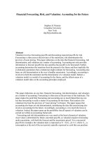
Accordingly the paper asks whether B/P adds to average return for a given E/P. The
table below summarizes the results from data using all U.S. listed stocks from 1963-2006.
______________________E/P Portfolio ._____
1 2 3 4 5
1 4.3% 10.9% 14.2% 17.1% 19.7%
B/P 2 8.8 9.1 13.0 16.0 22.1

Port- 3 14.4 8.5 12.1 17.0 21.6
folio 4 15.5 13.4 14.7 18.0 24.3
5 26.4 20.1 20.2 22.6 30.0
____________________________________________________________
To prepare this table, firms were ranked on their earnings/price (E/P) ratios each year
and grouped into the five portfolios indicated. Then, within each E/P portfolio, firms
were grouped into five B/P portfolios. Returns are then observed over the following 12
months. The table reports the average annual returns for each portfolio from replicating
these positions in each of the 44 years. Although significance tests have not been reported
here, it is clear that E/P ranks returns (across rows) as equation (9) suggests. However,
for a given E/P, the higher the B/P ratio (down columns), the higher the average return.
One can always attribute the result to market inefficiency, of course, but the “rational”
accounting interpretation can also be put on the table. The result for E/P suggests that
short-term earnings are at risk and the market prices them as such: more expected
earnings (relative to price) mean higher risk, consistent with the risk-return tradeoff. This
is not difficult to swallow. Investors surely see earnings at risk and casual evidence, let
alone much research, suggests that when firms’ actual earnings differ from expectation,
stock prices are shocked. The results for B/P further suggest that additional long-term
13

earnings are also at risk, consistent with the notion that growth is risky but also consistent
with the idea that accounting defers earnings to the future under uncertainty.
18

The results also explain the Fama and French B/P effect in stock returns, and in a way
that reconciles B/P as a risk attribute to accounting-based valuation. B/P is correlated
with E/P—the average rank correlation is 0.31(and 0.48 for positive E/P)—so part of the
B/P effect is due to short-term earnings risk. But B/P also indicates growth at risk. Note,
however, that the growth is quite different from the growth typically attributed to B/P,
where a low B/P (rather than a high B/P) is deemed to be “growth” (as opposed to

“value”).

Synthesis
The discussion has provided a synthesis of forecasting and accounting. Financial
forecasting for valuation involves accounting for the future, for accounting both specifies
what is to be forecasted and how the forecaster transitions from the present to the future.
The point opens up a number of research questions, most importantly the issue of what is
the appropriate accounting for the future.
The discussion on accounting, risk, and asset pricing is more conjectural. The reader is
asked to consider that accounting for the future that involves earnings deferral has
something to do with risk. (Accountants have no problem with the idea.) It opens the
question as to whether asset pricing models might be developed from the idea that
earnings and earnings growth are at risk. This is not an unreasonable suggestion, for
investors “buy earnings”, and typically see that earnings are at risk. The discussion here
has added some provocative accounting reasons to adopt this perspective.
Moreover, the perspective is supported by empirical research, reported here, that
provides an accounting rationale for the book-to-price effect in stock returns which has so
mystified researchers in asset pricing. Asset pricing models have been developed based
on the empirical regularity of the book-to-price effect but, without an explanation for the
effect, these models are ad hoc. The discussion in the paper here raises the question of
whether a pricing model can be developed from the notion that earnings and earnings
growth are at risk, but in a way that is consistent with the theory of no-arbitrage asset
pricing. If so, both aspects of valuation – forecasting and the discount for risk – will be
seen as a matter of accounting for the future.
Bringing together the ideas the paper, one appreciates that forecasting is a matter of
accounting and that accounting has the potential to be revealing about risk. All depends
on the accounting principles. For a given set of accounting principles, how does the
forecasting and risk revelation help or hinder valuation? How might an alternative
accounting be designed to enhance valuation and risk determination?
References

Ang, A., and J. Liu. 2001. A general affine earnings valuation model.
Review of
Accounting Studies
6, 397-425.

Ball, R., and R. Watts. 1972. Some time series properties of accounting income.
Journal
of Finance
27, 663-682.

18
The E/P and B/P stock screen has long been trolled by value-growth investors. The interpretation here
suggests that this trading strategy comes with risk.
14


Beaver, W., P. Kettler, and M. Scholes. 1970. The association between market
determined and accounting determined risk measures. The Accounting Review 45, 654-
682

Breeden, D., and R. Litzenberger. 1978. Prices of state-contingent claims implicit in
option prices. Journal of Business 51, 621-651.

Brief, R., and R. Lawson. 1992. The role of the accounting rate of return in
financial statement analysis. The Accounting Review 67, 411-426.

Christensen, P., and G. Feltham. 2009. Equity valuation. Foundations and Trends in
Accounting
4, 1-112.

Cohen, R., C. Polk, and T. Vuolteenaho. 2009. The price is (almost) right. Journal of
Finance
64, 2739-2782.

Courteau, L., J. Kao, and G. Richardson. 2001. Equity valuation employing the ideal
versus ad hoc terminal value expressions. Contemporary Accounting Research 18, 625-
661.

Easton, P, T. Harris, and J. Ohlson. 1992. Accounting earnings can explain most of
security returns: The case of long event windows. Journal of Accounting and
Economics 15, 119-142.
Feltham, J., and J. Ohlson. 1995. Valuation and Clean Surplus Accounting for Operating
and Financial Activities. Contemporary Accounting Research 11, 689-731.

Feltham, G., and J. Ohlson. 1999. Residual income valuation with risk and stochastic
interest rates. The Accounting Review 74, 165-183.

Francis, J., P. Olsson, and D. Oswald. 2000. Comparing the accuracy and explainability
of dividend, free cash flow, and abnormal earnings equity value estimates.
Journal of
Accounting Research
38, 45-70.

Freeman, R., J. Ohlson, and S. Penman. 1982. Book rate-of-return and prediction of
earnings changes: An empirical investigation.
Journal of Accounting Research 20, 639-
653.

Lintner, J., and R. Glauber. 1967. Higgledy piggledy growth in America. Paper presented
at the Seminar on the Analysis of Security Prices, University of Chicago, May 1967.

Lettau, M., and S. Ludvigson. 2005. Expected returns and expected dividend growth.
Journal of Financial Economics 76, 583-626.

Lücke,W. 1955. Investitionsrechnung auf der grundlage von ausgaben oder kosten?
15

Zeitschrift für Betriebswirtschaftliche Forschung, 310-324.

Lundholm, R., and T. O’Keefe. 2001a. Reconciling value estimates from the discounted
cash flow model and the residual income model.
Contemporary Accounting Research
18, 311-335.

Lundholm, R., and T. O’Keefe. 2001b. On comparing residual income and discounted
cash flow models of equity valuation: A response to Penman (CAR, Winter 2001).
Contemporary Accounting Research 18, 681-692.
Menzly, L., T. Santos, and P. Veronesi. 2004. Understanding Predictability.
Journal of
Political Economy 112, 1-47.

Nekrasov, A., and P. Shroff. 2009. Fundamentals-based risk measurement in valuation.

The Accounting Review 84, 1983-2011.

Nissim, D., and S. Penman. 2007.
Principles for the Application of Fair Value
Accounting

. White Paper No. 2, Center for Excellence in Accounting and Security
Analysis, Columbia Business School.
Ohlson, J. 1995. Earnings, book values, and dividends in equity valuation. Contemporary
Accounting Research
11, 661-687.

Ohlson, J. 2005. On accounting-based valuation formulae. Review of Accounting Studies
10, 323-347.

Ohlson, J. 2008. Risk, growth, and permanent earnings. Unpublished paper,
Arizona State University.

Ohlson, J., and X. Zhang. 1998. Accrual accounting and equity valuation. Journal of
Accounting Research
36 (Supplement), 85-111.

Peasnell, K. 1982. Some formal connections between economic values and yields and
accounting numbers.
Journal of Business Finance and Accounting 9, 361-381.

Penman, S. 1997. A synthesis of equity valuation techniques and the terminal value for
the dividend discount model. Review of Accounting Studies 2, 303-323.

Penman, S. 2001. On comparing cash low and accrual accounting models for use in
equity valuation: A response to Lundholm and O’Keefe (CAR, Summer 2001).
Contemporary Accounting Research 18, 681-692.
Penman, S. 2009. Accounting for intangible assets: There is also an income statement.
Abacus 45, 359-371.
Penman, S. 2010. Financial Statement Analysis and Security Valuation, 4
th

ed. New
York: The McGraw-Hill Companies.
Penman, S. and T. Sougiannis. 1998. A comparison of dividend, cash flow, and earnings
16

17

approaches to equity valuation. Contemporary Accounting Research 15, 343-383.

Penman, S., and F. Reggiani. 2008. Returns to buying earnings and book values:
Accounting for growth. Unpublished paper, Columbia University and Bocconi
University.

Penman, S., and X. Zhang. 2002. Accounting conservatism, the quality of earnings, and
stock returns. The Accounting Review 77, 237-264.

Penman, S., and X. Zhang. 2006. Modeling sustainable earnings and P/E ratios with
financial statement information. Unpublished paper, Columbia University and
University of California, Berkeley.

Preinreich, G. 1936. The fair value and yield of common stock.
The Accounting Review,
130-140.

Preinreich, G.1938. Annual survey of economic theory: The theory of depreciation.

Econometricia 6, 219-41.

Preinreich, G. 1941. Note on the theory of depreciation. Econometrica 9, 80-88,

Rosenberg. B., and V. Marathe. 1975. The prediction of investment risk: Systematic and
residual risk. Paper in the Proceedings of the Seminar on the Analysis of Security
Prices
, Graduate School of Business, University of Chicago.

Rubinstein, M. 1976. The valuation of uncertain income streams and the pricing of
options. Bell Journal of Economics 7, 407-425.

Thomas, J., and F. Zhang. 2009. Understanding two remarkable findings about stock
yields and growth. Journal of Portfolio Management, forthcoming.

Zhang, X. 2000. Conservative Accounting and Equity Valuation.
Journal of Accounting
and Economics
29, 125-149.