Control Systems Lab (SC4070)
Bạn đang xem bản rút gọn của tài liệu. Xem và tải ngay bản đầy đủ của tài liệu tại đây (28.63 KB, 1 trang )
Control Systems Lab (SC4070)
Inverted Wedge (Balance) Experiment
Description
Table 1: Physical parameters and their values.
The inverted wedge (also called balance) setup consists of
a cart driven by a DC motor. The motor can steer the cart
left and right on a track approximately one meter long. The
track itself can freely rotate in the plane coinciding with the
direction of motion of the cart. The objective is to control
the motion of the cart such that the track is balanced at a
desired angle. The schematic diagram in Figure 1 shows
the construction of the system including all the relevant parameters and variables. Positive directions of variables are
indicated by arrows.
g
b
α
m
M
J
km
b
Parameter
acceleration due to gravity
height of track
distance from center of
gravity to point of rotation
mass of cart
mass of balance
inertia of balance
input-to-force gain
damping coefficient
Value
9.81 ms−2
0.11 m
0.045 m
0.49 kg
3.3 kg
0.42 kgm2
5.0 N
4 to 10 kgs−1
Control Objective
km
d
u
m
a
c
Symbol
g
a
c
M, J
Figure 1: Schematic drawing of the inverted wedge.
This system has one control input u, which is the force
that accelerates the cart left or right (delivered by the motor). This input is commanded from the computer and is
scaled between -1 (corresponds to the maximal force moving the cart to the left) and +1 (corresponds to the maximal
force moving the cart to the right).
There are two measured outputs: d – the position of the
cart, and α – the angle of the track. These measurements
are given in their physical units – meters and radians, respectively.
The physical parameters of the system are listed in Table 1. Most of the values can easily be determined by measuring the dimensions and masses (such as the height of the
track, the mass of the cart, etc.). The input-to-force gain
km can be computed from the motor specifications and the
gains of the interface amplifiers.
The value of the damping coefficient b (including viscous friction and the back-emf of the motor) is not known
a priori and can only be determined experimentally (an estimated range is given in Table 1. It is your task to devise
and carry out an identification experiment to obtain a more
accurate value for this damping coefficient b.
Another parameter that cannot be accurately measured
is the distance from the center of gravity of the track to
the point of rotation c (the position of the center of gravity is unknown). Another identification experiment would
be needed to obtain an estimate for this parameter. As only
limited time is available in the lab, a reasonable value is already provided in Table 1. You may of course think about a
suitable experiment and if time permits you may verify the
given value.
Design a controller that makes the angle α of the balance
track follow a specified reference trajectory. The controlled
system should have zero steady state error in α and adequate disturbance rejection properties, i.e., it should be able
to recover from a small tick against the track.
Physical Modeling
The nonlinear model equations are given below. They have
been derived by using the Euler–Lagrange equations, neglecting rotational viscous friction, translational Coulomb
friction and stiction and the dynamics of the motor electrical circuit (armature).
1
km u − ma¨
α − bd˙ + mdα˙ 2 + mg sin(α)
(1)
d¨ =
m
1
−mad¨ − 2αmd
˙
d˙ + mga sin(α)
α
¨=
J + ma2 + md2
+ mgd cos(α) + M gc sin(α)
(2)
The term ma2 + md2 is a point mass approximation of the
added inertia due to the cart.
Note that α
¨ depends on d¨ and vice versa: this is called
an algebraic loop. Simulink will display warnings when you
simulate these equations and the simulation will be slower
(the algebraic loop must be solved numerically in each simulation step). It is therefore advised to break the algebraic
loop either by neglecting the term a¨
α in Equation 1 or by inserting a delay of one integration step (block called “Memory”, in the library of continuous-time blocks).
Simulink Template
A Simulink template baltemplate.mdl contains the
necessary real-time interface blocks and some scopes.
Make your own copy of this file and use it as a starting point
for your experiments. Before starting the first simulation,
define the sampling period h as a variable in the workspace
of M ATLAB. Always use the red button “Stop” to stop the
system before you terminate a simulation. Use the other
buttons to move the cart to a desired initial position.